A Comprehensive Guide to 16S rRNA Sequencing Sample Preparation: From DNA Extraction to Data Validation
This article provides a detailed guide for researchers and drug development professionals on 16S rRNA sequencing sample preparation, a critical step influencing data accuracy in microbiome studies.
A Comprehensive Guide to 16S rRNA Sequencing Sample Preparation: From DNA Extraction to Data Validation
Abstract
This article provides a detailed guide for researchers and drug development professionals on 16S rRNA sequencing sample preparation, a critical step influencing data accuracy in microbiome studies. Covering foundational principles to advanced applications, it explores DNA extraction optimization, library preparation for short and long-read platforms, primer selection to minimize bias, and troubleshooting for common pitfalls. The content also evaluates methodological performance across sequencing technologies and bioinformatic tools, offering evidence-based protocols for clinical diagnostics, environmental monitoring, and biomarker discovery to ensure reliable, reproducible results in biomedical research.
Understanding 16S rRNA Sequencing: Principles and Applications in Biomedical Research
Core Principles of 16S rRNA Gene as a Phylogenetic Marker
The 16S ribosomal RNA (rRNA) gene has established itself as the foremost molecular chronometer for microbial phylogenetics and taxonomy. This gene, encoding the RNA component of the 30S ribosomal subunit, provides an evolutionary framework for classifying and identifying bacteria and archaea, fundamentally transforming our understanding of microbial evolution and diversity [1] [2]. Its adoption as a standard marker pioneered by Woese and others in the 1970s enabled the revolutionary discovery of the three-domain system of life, categorizing cellular life into Bacteria, Archaea, and Eucarya [1] [2]. The application of 16S rRNA gene sequencing has subsequently become indispensable in clinical microbiology, environmental studies, and microbiome research, allowing researchers to identify poorly described, rarely isolated, or phenotypically aberrant strains that defy traditional culture-based techniques [1] [3].
The gene's critical advantage lies in its functional constancy coupled with appropriate sequence variability. As part of the protein synthesis machinery, the 16S rRNA molecule performs essential biological functions that constrain extensive mutation, leading to slow evolutionary rates and the preservation of recognizable homology across billions of years of evolutionary divergence [1] [4]. Simultaneously, the ~1,550 base-pair gene contains nine hypervariable regions (V1-V9) that are flanked by conserved stretches, creating a molecular signature with sufficient interspecific polymorphisms to discriminate between taxonomic groups while providing universal primer binding sites for PCR amplification across broad phylogenetic ranges [1] [5] [4]. This combination of universal distribution, functional conservation, and measured variability solidifies the 16S rRNA gene's position as the cornerstone of modern microbial phylogenetics.
Core Structural and Functional Properties
Molecular Architecture
The 16S rRNA gene exhibits a sophisticated architectural design that directly enables its utility as a phylogenetic marker. The gene's approximately 1,500-nucleotide sequence folds into a complex secondary and tertiary structure containing about 50 functional domains that are critical for ribosomal assembly and protein synthesis [6] [4]. These structural elements include the immobilization of ribosomal proteins as scaffolding, a reverse SD sequence at the 3' end that binds to the AUG initiation codon of mRNA, and interaction sites that help integrate the 30S and 50S ribosome subunits [4].
The gene's sequence organization features highly conserved regions interspersed with nine hypervariable regions (V1-V9) that range from 30-100 base pairs in length [5] [4]. The conserved regions maintain the ribosome's essential functional integrity across all bacterial lineages, while the variable regions accumulate nucleotide substitutions at different rates, creating unique signatures for different taxonomic groups [1] [3]. This structural arrangement permits the design of universal PCR primers targeting the conserved areas, enabling amplification of the intervening variable regions that provide taxonomic discrimination power [3] [4].
Phylogenetic Signal Characteristics
The 16S rRNA gene serves as an exceptional molecular chronometer that records evolutionary distance and relatedness among organisms [1]. Several key properties make it ideally suited for phylogenetic analysis:
- Universal Distribution: The 16S rRNA gene is present in all known bacteria and archaea, allowing comparative analysis across all major phylogenetic lineages [1] [3].
- Multiple Copy Number: Most bacteria contain 5-10 copies of the 16S rRNA gene in their genomes, enhancing detection sensitivity in molecular assays [4].
- Appropriate Evolutionary Rate: The gene exhibits a relatively slow but measurable rate of sequence divergence, preserving recognizable homology across deep evolutionary divisions while accumulating sufficient variation for distinguishing recently diverged lineages [1] [3].
- Minimal Horizontal Transfer: As part of the core ribosomal machinery, the 16S rRNA gene rarely undergoes horizontal gene transfer, ensuring that phylogenetic relationships reflect organismal evolutionary history [1].
Table 1: Key Characteristics of the 16S rRNA Gene as a Phylogenetic Marker
| Property | Description | Phylogenetic Utility |
|---|---|---|
| Length | ~1,550 base pairs | Provides sufficient sequence information for robust statistical analysis |
| Copy Number | 1-21 copies per genome (typically 5-10) | Enhances PCR detection sensitivity; requires correction for quantitative studies [7] |
| Conserved Regions | 9 segments with minimal sequence variation | Enables design of universal PCR primers across broad taxonomic ranges |
| Variable Regions | 9 hypervariable regions (V1-V9) | Provides taxonomic discrimination at multiple phylogenetic levels |
| Evolutionary Rate | Slow but measurable divergence | Functions as a reliable molecular chronometer for deep and shallow relationships |
Experimental Methodology and Workflow
Sample Preparation and DNA Extraction
The initial phase of 16S rRNA analysis requires careful sample preparation to obtain high-quality microbial DNA suitable for PCR amplification. The selection of DNA extraction method depends critically on sample type, as different matrices present unique challenges for cell lysis and DNA purification. For environmental water samples, the ZymoBIOMICS DNA Miniprep Kit provides effective recovery of diverse community DNA. For complex matrices like soil samples, the QIAGEN DNeasy PowerMax Soil Kit is recommended due to its capacity to remove PCR-inhibiting humic substances. For stool samples representative of human microbiomes, either the QIAamp PowerFecal DNA Kit for microbiome-specific DNA or the QIAGEN Genomic-tip 20/G for a balanced host-microbiome DNA mixture are appropriate choices [5].
The DNA extraction process must be tailored to the bacterial groups present in the sample. For instance, Gram-positive bacteria with robust cell walls often require additional lysis steps, such as treatment with achromopeptidase (incubation for 1 hour at 37°C) to ensure complete disruption [8]. Subsequent steps typically involve proteinase K digestion (40 μl with 180 μl ATL buffer at 55°C for 1 hour) followed by a final lysis step with AL buffer (incubation at 70°C for 10 minutes) [8]. The quality and quantity of extracted DNA should be rigorously assessed using fluorometric methods (e.g., Qubit dsDNA HS Assay) rather than spectrophotometry, as the former provides more accurate quantification of double-stranded DNA without contamination interference [8].
PCR Amplification and Library Preparation
Targeted amplification of the 16S rRNA gene represents the most critical step in preparing sequencing libraries. Primer selection determines which variable regions will be sequenced and ultimately governs the taxonomic resolution achievable in downstream analyses. Most commonly targeted regions include V3-V4 (~428 bp), V4 (~252 bp), and V1-V3 (~510 bp), with each offering different trade-offs between taxonomic discrimination, amplicon length, and sequencing platform compatibility [6] [4] [2].
For the V3-V4 hypervariable regions, which provide a balanced solution for species-level identification and Illumina sequencing compatibility, researchers can use primers Pro341F (5'-CCTACGGGNBGCASCAG-3') and Pro805R (5'-GACTACNVGGGTATCTAATCC-3') [8]. PCR amplification should be performed using a high-fidelity polymerase such as iProof (Bio-Rad) with the following cycling conditions: initial denaturation at 95°C for 3 minutes, followed by 35 cycles of 95°C for 30 seconds, 55°C for 30 seconds, 72°C for 30 seconds, and a final extension at 72°C for 5 minutes [8]. The inclusion of barcoded primers, such as those provided in the 16S Barcoding Kit (Oxford Nanopore), enables multiplexing of up to 24 samples in a single sequencing run, significantly reducing per-sample costs [5].
Following amplification, PCR products must be purified to remove primers, enzymes, and non-specific amplification products, then quantified before pooling in equimolar ratios for library preparation. The quality of amplicons should be verified by agarose gel electrophoresis to confirm the expected product size and absence of primer dimers or non-specific amplification [8].
Figure 1: 16S rRNA Gene Analysis Workflow. The complete experimental and computational pipeline from sample collection through to diversity analysis.
Sequencing Platform Selection
The choice of sequencing platform dictates whether partial or full-length 16S rRNA gene sequences can be obtained, significantly impacting taxonomic resolution. Second-generation platforms like Illumina MiSeq typically sequence shorter reads (≤300 bp) covering 1-2 variable regions, while third-generation platforms like Oxford Nanopore and Pacific Biosciences can generate reads spanning the entire ~1,500 bp gene [5] [4].
Table 2: Sequencing Platforms and Their Compatible 16S rRNA Gene Regions
| Sequencing Platform | Common Target Regions | Approximate Length | Resolution Considerations |
|---|---|---|---|
| Illumina MiSeq | V3-V4 | ~428 bp | Good for genus-level, some species-level discrimination |
| Illumina HiSeq | V4 | ~252 bp | Cost-effective for large studies, limited species resolution |
| Roche 454 | V1-V3, V3-V5, V6-V9 | ~510 bp, ~428 bp, ~548 bp | No longer widely available, historical data compatibility |
| Pacific Bioscience | V1-V9 (full-length) | ~1,500 bp | Maximum taxonomic resolution to species level |
| Oxford Nanopore | V1-V9 (full-length) | ~1,500 bp | Real-time sequencing, species-level identification from polymicrobial samples [5] |
Full-length 16S rRNA gene sequencing provides superior taxonomic resolution, particularly for discriminating between closely related species that may share identical sequences in commonly targeted subregions [5]. For Oxford Nanopore full-length sequencing, researchers should employ the high-accuracy (HAC) basecaller in MinKNOW software and sequence for approximately 24-72 hours to achieve 20x coverage per microbe in multiplexed libraries [5]. Flow cells not run at full capacity can be washed and reused multiple times using the Flow Cell Wash Kit, providing cost-efficiency for smaller batches [5].
Bioinformatics Analysis Pipeline
Data Processing and Quality Control
Raw sequencing data requires substantial preprocessing before biological interpretation can begin. The initial quality control steps involve filtering sequences based on quality scores, removing ambiguous base calls, and eliminating chimeric sequences generated during PCR amplification through algorithms like USEARCH or UCHIME [6] [2]. For paired-end Illumina sequences, overlapping reads should be joined using tools like fastq-join to create longer, more informative amplicon sequences [2].
Two principal approaches exist for resolving biological sequences from the processed reads: Operational Taxonomic Units (OTUs) and Amplicon Sequence Variants (ASVs). OTU clustering groups sequences based on similarity thresholds (typically 97% for species-level groupings), while ASV methods (e.g., DADA2) differentiate sequences that vary by even a single nucleotide, providing higher resolution without relying on arbitrary similarity thresholds [6] [2]. The DADA2 algorithm implemented in QIIME2 performs particularly well for denoising, dereplication, and chimera removal, producing a feature table of unique sequence variants and their counts across samples [6].
Taxonomic Classification and Diversity Analysis
Taxonomic assignment involves comparing processed sequences against curated 16S rRNA reference databases using classification algorithms. Commonly employed databases include:
- SILVA: Comprehensive, regularly updated database of aligned ribosomal RNA sequences [6] [2]
- Greengenes: 16S rRNA gene database with quality-checked, chimera-checked sequences [6]
- RDP (Ribosomal Database Project): High-quality, annotated bacterial and archaeal 16S rRNA sequences [2]
- HOMD (Human Oral Microbiome Database): Specialized database for oral microorganisms [6]
Classification is typically performed using a naive Bayesian classifier implemented in tools like QIIME2 or the DADA2 package, which assigns taxonomy based on sequence similarity to reference sequences with known taxonomic affiliations [6] [2]. The confidence threshold for taxonomic assignments should be optimized based on the specific variable region sequenced and the required phylogenetic resolution.
Microbial community analysis employs two fundamental diversity metrics: alpha diversity, measuring richness and evenness within a single sample, and beta diversity, quantifying compositional differences between samples [6] [2]. Alpha diversity is commonly assessed using indices like Shannon, Chao1, or Observed Species, while beta diversity employs distance metrics such as Bray-Curtis dissimilarity, Jaccard distance, or phylogenetically-informed UniFrac distances [6] [2]. These analyses are typically implemented in R packages like phyloseq, which integrates the various components of amplicon sequencing data (taxonomy table, count data, phylogenetic tree, sample metadata) into a unified analysis framework [6].
Research Reagent Solutions and Materials
Table 3: Essential Research Reagents for 16S rRNA Gene Analysis
| Reagent/Kits | Specific Examples | Function/Purpose |
|---|---|---|
| DNA Extraction Kits | ZymoBIOMICS DNA Miniprep Kit (water samples), QIAGEN DNeasy PowerMax Soil Kit (soil), QIAamp PowerFecal DNA Kit (stool) | Sample-specific optimized DNA extraction and purification [5] |
| PCR Enzymes | iProof High-Fidelity Polymerase (Bio-Rad) | High-fidelity amplification of 16S rRNA gene targets with low error rates [8] |
| 16S Amplification Primers | Pro341F/Pro805R (V3-V4 region), 27F/1492R (full-length) | Target-specific amplification of hypervariable regions with universal coverage [5] [8] |
| Library Preparation | 16S Barcoding Kit 24 (Oxford Nanopore) | PCR amplification with barcoded primers for multiplex sequencing [5] |
| Quantification Assays | Qubit dsDNA HS Assay (Invitrogen) | Accurate quantification of double-stranded DNA for library normalization [8] |
| Positive Controls | Zymo Mock Microbial Community | Verification of PCR, extraction, and sequencing efficacy [6] |
Applications and Limitations in Modern Research
Key Research Applications
The 16S rRNA gene sequencing approach has enabled transformative applications across multiple research domains:
Clinical Diagnostics: Rapid identification of bacterial pathogens directly from clinical specimens, including unculturable or fastidious organisms, enabling evidence-based antibiotic therapy and detection of novel pathogens [1] [3]. The method is particularly valuable for identifying clinically unidentifiable bacterial isolates that resist conventional phenotypic characterization [3].
Microbiome Research: Comprehensive profiling of human-associated microbial communities at various body sites, revealing correlations between microbiota composition and health status, disease conditions, or therapeutic interventions [6] [3]. The approach has illuminated the critical role of host-microbiome interactions in conditions ranging from metabolic disorders to neurological diseases [6].
Environmental Microbiology: Characterization of microbial communities in diverse habitats including soil, water, extreme environments, and industrial systems, enabling monitoring of ecosystem health, bioremediation potential, and biogeochemical cycling [3].
Biotechnological Screening: Identification of novel bacterial strains with potential industrial applications, including producers of antimicrobial compounds, enzymes, and other bioactive molecules from environmental samples [9].
Current Limitations and Considerations
Despite its widespread utility, 16S rRNA gene analysis presents several important limitations that researchers must consider:
Variable Taxonomic Resolution: The method cannot reliably distinguish between certain closely related species that share nearly identical 16S rRNA gene sequences, such as some Bacillus and Streptomyces species [9] [2]. In the Streptomyces genus, distinct species may share identical full-length 16S sequences, while isolates belonging to the same species may contain different 16S rRNA sequences [9].
Gene Copy Number Variation: Different bacterial genomes contain varying copies of the 16S rRNA gene (ranging from 1 to 21 copies), creating quantitative bias where taxa with higher copy numbers are overrepresented in amplicon counts relative to their actual abundance [7] [10]. Correction methods using tools like PICRUSt, CopyRighter, or PAPRICA show limited predictive accuracy, particularly for taxa distantly related to sequenced reference genomes [10].
Database-Dependent Accuracy: Taxonomic assignments are only as reliable as the reference databases used, with misannotations in public databases potentially propagating errors in sample classification [1] [9].
Primer Selection Bias: No single primer pair truly captures all bacterial lineages equally, with certain taxa (e.g., Actinobacteria and Bifidobacteria) exhibiting significant polymorphism in primer binding regions that leads to their underrepresentation [2].
Functional Inference Limitations: While tools like PICRUSt attempt to predict functional potential from 16S data, these inferences are indirect and less reliable than metagenomic approaches for characterizing community functional capacity [2].
Emerging Methodological Advances
Recent technological innovations are addressing several traditional limitations of 16S rRNA gene analysis:
Full-Length Sequencing: Third-generation sequencing platforms from Oxford Nanopore and Pacific Biosciences now enable sequencing of the entire ~1,500 bp 16S rRNA gene, providing enhanced taxonomic resolution compared to short-read approaches targeting individual variable regions [5] [4].
Machine Learning Applications: Deep learning approaches like ANNA16 (Artificial Neural Network Approximator for 16S rRNA gene copy number) demonstrate improved prediction of 16S gene copy numbers directly from sequence data, potentially enabling more accurate quantitative corrections in community profiling [7].
Integrated Multi-omics: Combining 16S rRNA profiling with metagenomic, metatranscriptomic, and metabolomic approaches provides a more comprehensive understanding of microbial community structure and function, bridging the gap between taxonomic composition and biological activity [2].
Improved Reference Databases: Curated databases with better taxonomic annotations and expanded representation of previously uncultured lineages continue to enhance classification accuracy and discovery of novel taxa [6] [9].
As these methodological advances mature, 16S rRNA gene analysis will maintain its essential role in microbial ecology and clinical microbiology while providing increasingly accurate and comprehensive insights into the microbial world.
The 16S ribosomal RNA (rRNA) gene is a approximately 1,500 base-pair genetic sequence that functions as a cornerstone for microbial classification and identification [5] [4]. This gene contains nine hypervariable regions (V1-V9) that are flanked by highly conserved sequences [5] [11]. The conserved regions allow for the design of universal PCR primers, while the variable regions provide the species-specific signature necessary for taxonomic discrimination [4]. The 16S rRNA gene is present in all bacteria and archaea, and its multi-copy nature within genomes enhances detection sensitivity, making it an ideal target for sequencing-based microbial community analysis [12] [4].
For decades, technological constraints limited sequencing to short fragments of the 16S rRNA gene, typically one to several hypervariable regions [11]. However, the advent of third-generation sequencing technologies, such as those offered by Oxford Nanopore Technologies (ONT) and PacBio, has enabled routine full-length 16S rRNA gene sequencing [5] [13]. This advancement overcomes the resolution limitations of short-read platforms, as sequencing the entire gene provides a greater density of taxonomic information, leading to more accurate and precise microbial identification, often at the species level [11] [14]. This Application Note details the protocols and key applications of full-length 16S rRNA sequencing across clinical and environmental fields.
Comparative Performance of Sequencing Approaches
The transition from short-read to long-read sequencing represents a significant evolution in microbiome analysis. Table 1 summarizes the key differences between these approaches, highlighting the advantages of full-length 16S sequencing.
Table 1: Comparison of Short-Read vs. Long-Read 16S rRNA Sequencing
| Feature | Short-Read Sequencing (e.g., Illumina) | Long-Read Sequencing (e.g., ONT, PacBio) |
|---|---|---|
| Target Region | Partial gene (e.g., V3-V4, V4) [11] | Full-length gene (V1-V9) [5] [11] |
| Taxonomic Resolution | Primarily genus-level [11] [15] | Species- and strain-level possible [11] [14] |
| Primary Challenge | Region selection bias; cannot resolve closely related species [11] | Higher per-read error rates, though now >99% accurate [14] [13] |
| Throughput & Cost | High throughput, established lower cost per sample | Rapid, real-time results; scalable and cost-effective for individual samples [15] |
| Ideal For | Large-scale genus-level diversity studies | Diagnostics, strain tracking, and high-resolution community profiling [16] [14] |
Recent studies validate the performance of long-read sequencing. A 2025 clinical evaluation demonstrated that ONT sequencing had significantly higher taxonomic resolution at the genus level compared to Sanger sequencing, with 91% species-level concordance when both methods achieved species identification [14]. In environmental science, a 2025 study on soil microbiomes found that ONT and PacBio provided comparable assessments of bacterial diversity, with both platforms clearly clustering samples by soil type, a result not achieved by sequencing only the V4 region [13].
Application Notes & Experimental Protocols
Clinical Diagnostics: Pathogen Identification from Isolates
Application Note: In clinical microbiology, 16S rRNA sequencing is a critical tool for identifying bacterial pathogens that yield ambiguous biochemical profiles or cannot be identified by proteomic methods like MALDI-TOF MS [14]. The full-length gene sequencing approach is particularly valuable for distinguishing between closely related species where diversity does not occur within the first 500 bp typically sequenced by Sanger methods [14].
Experimental Protocol:
Sample Collection & DNA Extraction:
- Collect bacterial isolate from a pure culture.
- Extract genomic DNA using a dedicated kit such as the Quick-DNA Fungal/Bacterial Miniprep kit (Zymo Research) [14]. Boil-prep extraction methods should be avoided as they can interfere with nanopore sequencing [14].
- Quantify DNA concentration using a fluorometer (e.g., Qubit) and assess purity via spectrophotometer (e.g., NanoDrop) to ensure a 260/280 ratio of ~1.8 [14].
Library Preparation:
- Use the 16S Barcoding Kit (SQK-16S024) from Oxford Nanopore Technologies according to manufacturer instructions [5] [14].
- Amplify the full-length ~1.5 kb 16S rRNA gene from 50 ng of gDNA using barcoded primers (e.g., 27F and 1492R) in a PCR reaction [5] [16].
- Purify the PCR amplicons and attach sequencing adapters.
Sequencing:
Data Analysis:
- Perform basecalling and demultiplexing in real-time using MinKNOW or post-run using Guppy.
- For taxonomic classification, use curated databases and analysis pipelines. The EPI2ME wf-16s workflow from ONT provides a user-friendly option [5]. Alternatively, third-party software like the SmartGene IDNS with its proprietary 16S Centroid database has been clinically validated for high-accuracy species-level identification [14].
Environmental Monitoring: Soil Microbiome Profiling
Application Note: Characterizing soil microbial communities is essential for understanding ecosystem functioning, agricultural productivity, and biogeochemical cycling [13]. Full-length 16S sequencing enables researchers to move beyond coarse taxonomic profiles to species-level assessments, revealing subtle shifts in community structure in response to environmental changes [13].
Experimental Protocol:
Sample Collection & Storage:
DNA Extraction:
- Use a soil-specific DNA extraction kit such as the QIAGEN DNeasy PowerMax Soil Kit or the Quick-DNA Fecal/Soil Microbe Microprep Kit (Zymo Research) to efficiently lyse robust environmental microbes and co-purify inhibitors [5] [13].
- Validate extraction efficiency and DNA quality using a fluorometer and gel electrophoresis.
Library Preparation & Sequencing:
- Amplify the full-length 16S rRNA gene using universal primers (e.g., 27F: AGAGTTTGATYMTGGCTCAG and 1492R: GGTTACCTTGTTAYGACTT) [13].
- Purify amplicons using magnetic beads (e.g., KAPA HyperPure Beads) [13].
- Prepare the library using a multiplexing kit like the Native Barcoding Kit 96 (ONT) to pool multiple samples, reducing cost per sample [5] [13].
- Sequence on a MinION flow cell for ~24-48 hours. Flow cells can be washed and reused multiple times using a Wash Kit to further reduce costs for environmental monitoring projects [5].
Data Analysis:
- Process raw FASTQ files through a bioinformatics pipeline. Quality filter reads (e.g., Q-score ≥7, length 1,000-1,800 bp) [17].
- For taxonomic profiling, use tools like Emu, which is designed for long-read 16S data and generates fewer false positives [13] [17].
- Perform downstream ecological analyses (alpha/beta diversity, differential abundance) using tools like QIIME 2 or Phyloseq in R, comparing against comprehensive databases like SILVA [18].
Food Microbiology: Quality Control and Safety
Application Note: 16S metabarcoding is used to characterize the microbiome of food products, enabling the monitoring of spoilage organisms, starter cultures, and foodborne pathogens in a culture-independent manner [18]. This is particularly useful for complex or novel food matrices, such as insect-based products, where traditional culture methods may be inadequate [18].
Protocol Considerations:
- Sample Handling: Aseptic technique is critical during sampling to avoid contamination. Samples should be homogenized in a buffered peptone solution and either processed immediately or stored at -80°C [12].
- Database Selection: The choice of reference database significantly impacts results. For food microbiome analysis, the SILVA database has been shown to assign a significantly higher percentage of Amplicon Sequence Variants (ASVs) to the family and genus levels compared to RDP or RefSeq [18]. It is recommended to use the latest, curated version of the SILVA database for taxonomic assignment.
The Scientist's Toolkit: Key Reagent Solutions
Successful 16S rRNA sequencing relies on a suite of trusted reagents and tools. Table 2 catalogs essential solutions for the featured experiments.
Table 2: Essential Research Reagents and Tools for 16S rRNA Sequencing
| Item Name | Function / Application | Example Product / Vendor |
|---|---|---|
| DNA Extraction Kits | Isolate high-quality, inhibitor-free DNA from diverse sample types. | ZymoBIOMICS DNA Miniprep Kit (water) [5], QIAGEN DNeasy PowerMax Soil Kit (soil) [5], Quick-DNA Fungal/Bacterial Miniprep Kit (clinical isolates) [14] |
| 16S Amplification & Barcoding Kit | Amplify the full-length 16S gene and add sample-specific barcodes for multiplexing. | 16S Barcoding Kit 24 (SQK-16S024, Oxford Nanopore Technologies) [5] [14] |
| Sequencing Flow Cells | The consumable device where nanopore sequencing occurs. | MinION Flow Cells (Oxford Nanopore Technologies), compatible with MinION and GridION devices [5] |
| Flow Cell Wash Kit | Enables flow cell wash and reuse, reducing cost per sample. | Flow Cell Wash Kit (Oxford Nanopore Technologies) [5] |
| Internal Controls (Spike-ins) | Distinguishing absolute from relative abundance; quantifying microbial load. | ZymoBIOMICS Spike-in Control I (Zymo Research) [17] |
| Bioinformatics Databases | Reference databases for taxonomic classification of 16S sequences. | SILVA [18], SmartGene 16S Centroid [14], Greengenes [18] |
| Analysis Pipelines & Software | Process raw sequencing data into taxonomic and diversity metrics. | EPI2ME wf-16s (ONT) [5], Emu [13] [17], SmartGene IDNS [14] |
Critical Factors for Experimental Success
- Primer Selection: Primer choice is a major source of bias. A 2025 study on oropharyngeal swabs demonstrated that a more degenerate 27F primer (27F-II) yielded significantly higher alpha diversity and detected a broader range of taxa compared to the standard ONT 27F primer, aligning more closely with population-level reference data [16]. Recommendation: Use degenerate primers where possible to maximize inclusivity.
- Quantitative Accuracy: Standard 16S sequencing provides relative abundance data. For absolute quantification, essential in clinical load monitoring, incorporate internal spike-in controls (e.g., ZymoBIOMICS Spike-in) at the DNA extraction or PCR stage to correct for technical variation and enable load estimation [17].
- Contamination Control: The sensitivity of 16S PCR makes it vulnerable to contamination from reagents and the environment. Always process negative extraction controls (NECs) and no-template PCR controls in parallel with samples. The quantitative data from spike-ins and NECs can be used to subtract background contaminant DNA [15] [17].
- Database Curation: The accuracy of taxonomic identification is directly dependent on the quality and breadth of the reference database. Use well-curated, frequently updated databases like SILVA or the SmartGene Centroid database, which undergo rigorous quality control and annotation, for reliable results [14] [18].
Full-length 16S rRNA sequencing using long-read technologies has matured into a robust and essential method for microbial community analysis. Its applications span from delivering rapid, species-level pathogen identification in clinical diagnostics to providing high-resolution insights into complex environmental and industrial microbiomes. By adhering to optimized protocols for sample-specific DNA extraction, utilizing degenerate primers, incorporating internal controls for quantification, and leveraging curated bioinformatics databases, researchers can fully harness the power of this technology to advance scientific discovery and applied microbial surveillance.
The accuracy of 16S rRNA gene sequencing in characterizing microbial communities is highly dependent on the quality of the initial sample preparation. In the context of a broader thesis on 16S rRNA sequencing methodologies, this application note addresses the critical considerations for preparing diverse sample types, which vary dramatically in microbial biomass, complexity, and potential contaminants. While high-biomass samples like stool and soil present challenges in DNA extraction due to inhibitors and diverse cell structures, low-biomass specimens such as sterile body fluids and air are exceptionally vulnerable to contamination, where exogenous DNA can vastly exceed the target biological signal [19] [20]. This document provides detailed, sample-specific protocols and data-driven recommendations to ensure the integrity and reproducibility of microbiome data across these critical sample types, forming a foundational pillar for robust sequencing research.
Sample-Specific Challenges and Comparative Analysis
The inherent properties of different sample types directly influence the major challenges encountered during 16S rRNA sequencing workflows. The table below summarizes the primary obstacles and key mitigation strategies for each category.
Table 1: Critical Challenges and Mitigation Strategies for Different Sample Types in 16S rRNA Sequencing
| Sample Type | Key Challenges | Primary Mitigation Strategies |
|---|---|---|
| Stool | Presence of PCR inhibitors; Complex cell wall structures of Gram-positive bacteria [21] [12] | Boiling-based direct lysis; Column-free DNA extraction; Use of specialized inhibitor removal kits [21] |
| Soil | High abundance of humic acids and other PCR inhibitors; Extreme microbial diversity [22] | Validation of DNA extraction kits for inhibitor removal (e.g., DNeasy PowerSoil Pro Kit, FastDNA SPIN Kit for Soil) [22] |
| Sterile Fluids & Low-Biomass | Contamination from reagents, environment, and cross-sample "spill-over"; Approaching limits of detection [19] [20] | Rigorous contamination controls (NTCs, extraction blanks); Use of DNA-free reagents; PPE; Dedicated low-biomass workspace; In silico decontamination (e.g., decontam R package) [19] [20] |
The following workflow diagram outlines the core steps, with critical branching points, for processing these diverse sample types.
Detailed Experimental Protocols
Protocol for Fecal Sample Processing
This protocol is adapted from a guided, column-free method designed for high-throughput, reproducible profiling of gut microbiota [21].
- Sample Collection and Storage: Collect a smear of approximately 5 mm² from a fresh fecal sample using a sterile swab and place it in a collection tube. Store samples at -80°C within 24 hours of collection [21].
- DNA Extraction:
- Transfer the fecal swab to a 2 mL collection tube, trimming the stick if necessary for closure.
- Add 250 μL of Extraction Solution (e.g., containing LiCl, Tris-HCl, SDS, EDTA) and vortex to mix.
- Lyse cells by heating for 10 minutes in a boiling water bath (95–100°C).
- Add 250 μL of Dilution Solution, vortex to mix, and store the extracted DNA at 4°C [21].
- PCR Amplification and Library Preparation:
- In a clean, amplicon-free PCR workstation, prepare a PCR master mix. For a 20 μL reaction, use 15 μL of a mix containing forward primer, 2X PCR master mix, and water. Add 1 μL of a uniquely barcoded reverse index primer to each well.
- Add 4 μL of extracted DNA to the reaction mixture. Perform amplification in triplicate.
- PCR Conditions: Initial denaturation at 94°C for 3 min; 35 cycles of denaturation (94°C for 1 min), annealing (55°C for 1 min), and extension (72°C for 1 min); final extension at 72°C for 10 min.
- Combine the triplicate PCR reactions and verify amplicon size (e.g., ~400 bp for V4 region) on an agarose gel.
- Pool equimolar amounts of each sample (e.g., 500 ng each), perform gel extraction to isolate the correct band, and measure the final library concentration and size [21].
Protocol for Soil and Plant Root Samples
This protocol emphasizes high-throughput and effective removal of environmental inhibitors [22].
- Sample Homogenization: Cool root or soil samples with liquid nitrogen and immediately grind to a fine powder using a bead beater.
- DNA Extraction with Magnetic Beads:
- Transfer 500 mg of powdered sample to a tube and add 1 mL of Lysate Binding Buffer (e.g., containing LiCl, Tris-HCl, SDS, EDTA, DTT).
- Vortex, incubate at room temperature for 5 minutes, and centrifuge at 15,000 rpm for 10 minutes.
- Transfer the supernatant (LBB lysate) to a new tube.
- For high-throughput, add AMPure XP magnetic beads to the LBB lysate to bind DNA. Wash and elute the DNA.
- Library Preparation with Two-Step PCR: This method reduces bias compared to single-step PCR.
- First PCR: Amplify the target 16S region with gene-specific primers.
- Purification: Purify the first PCR product using exonuclease treatment to remove residual primers, which has been shown to capture higher microbial diversity compared to magnetic bead clean-up alone.
- Second PCR: Amplify the purified product with full-length primers containing sequencing adapters and sample barcodes [22].
Protocol for Low-Biomass and Sterile Fluids
This protocol is critical for samples where contaminating DNA can exceed the true signal [19] [23] [20].
- Contamination-Conscious Sampling:
- Decontaminate Sources: Use single-use, DNA-free collection vessels. Decontaminate reusable equipment with 80% ethanol followed by a nucleic acid degrading solution (e.g., bleach, UV-C light).
- Use Personal Protective Equipment (PPE): Wear gloves, masks, and clean suits to limit sample exposure to human-associated contaminants.
- Collect Controls: Include multiple negative controls such as empty collection vessels, swabs of the air, sampling fluids, and DNA extraction blanks [19].
- DNA Extraction and Sequencing:
- Use DNA extraction kits validated for low-biomass samples (e.g., QIAamp BiOstic Bacteremia DNA Kit for body fluids).
- For very low inputs, increase the PCR cycle number (e.g., to 35 cycles) to improve sensitivity, acknowledging the potential for increased bias.
- When using technologies like Nanopore sequencing for rapid diagnosis, determine a Threshold of Relative Abundance (TRA) via ROC analysis to distinguish true pathogens from background noise. For monomicrobial infections, a TRA of ~0.058 has been demonstrated effective [23].
The Scientist's Toolkit: Key Reagent Solutions
The selection of appropriate reagents is fundamental to success. The following table catalogues essential materials and their functions.
Table 2: Essential Research Reagents for 16S rRNA Sequencing Sample Preparation
| Reagent / Kit | Sample Application | Function and Rationale |
|---|---|---|
| ZymoBIOMICS DNA Miniprep Kit | Stool, Environmental Water [5] [20] | DNA extraction with proven efficacy for microbial lysis and inhibitor removal. |
| DNeasy PowerSoil Pro Kit / FastDNA SPIN Kit for Soil | Soil, Plant Roots [22] | Specifically formulated to remove humic acids and other potent PCR inhibitors from complex environmental samples. |
| QIAamp BiOstic Bacteremia DNA Kit | Sterile Body Fluids (Blood, CSF) [23] | Optimized for extracting microbial DNA from clinical, low-biomass specimens with high human DNA background. |
| AMPure XP Beads | Universal [21] [22] | Magnetic beads for high-throughput DNA clean-up and size selection, replacing column-based methods. |
| PrimeStore Molecular Transport Medium | Low-Biomass (Nasopharyngeal, Sputum) [20] | Sample storage buffer that yields lower background OTUs compared to other buffers like STGG, preserving sample integrity. |
| ZymoBIOMICS Microbial Community Standard | Universal Quality Control [22] [20] | Mock community with known composition; essential for validating DNA extraction efficiency, PCR bias, and sequencing accuracy. |
| 16S Barcoding Kit (e.g., SQK-16S024) | Universal Library Prep [23] [5] | Contains primers for full-length 16S amplification and barcodes for multiplexing samples on sequencing platforms like Nanopore. |
Data Analysis and Validation
For low-biomass studies, standard bioinformatic pipelines must be supplemented with robust contamination identification tools.
- In Silico Decontamination: Tools like the
decontampackage in R (using the "prevalence" method) can statistically identify and remove contaminant sequences by comparing their prevalence in experimental samples to their prevalence in negative controls. This is superior to simply subtracting control profiles, which can remove true biological signals [20]. - Bioinformatic Pipelines: Standard pipelines such as QIIME 2 (featuring DADA2 for sequence variant calling) or specific cloud-based platforms like EPI2ME for Nanopore data are widely used [21] [5]. It is critical to apply consistent sequence quality filtering and taxonomy assignment parameters across all samples in a study.
- Validation with Mock Communities: The inclusion of a known mock community in every sequencing run is non-negotiable for validating data quality. It allows researchers to assess sequencing error rates, confirm expected taxa, and measure overall reproducibility [24] [20].
Impact of Sample Preparation on Downstream Taxonomic Resolution
Within the framework of 16S rRNA sequencing sample preparation research, it is well-established that the methods employed during the pre-sequencing phase are not merely procedural steps but are critical determinants of data quality and biological interpretation. The goal of achieving high taxonomic resolution—the ability to accurately classify microorganisms to the species or even strain level—is heavily influenced by choices made long before sequencing begins. This application note details how specific sample preparation protocols, from nucleic acid extraction to primer selection and library construction, directly impact downstream taxonomic classification. We provide validated methodologies and quantitative data to guide researchers in optimizing these steps for more precise microbial community analysis.
The Critical Role of the Targeted 16S rRNA Gene Region
The selection of which variable region(s) of the 16S rRNA gene to amplify is one of the most significant preparative decisions, with a direct and quantifiable impact on taxonomic resolution.
Comparative Performance of Variable Regions
Table 1: Taxonomic Resolution of Different 16S rRNA Variable Regions [25]
| Target Region | Best-Performing Genera (Example) | Performance Notes |
|---|---|---|
| V1-V3 | Cupriavidus, Bacillus, Pseudomonas |
Demonstrated the best resolving power for 8 out of 16 plant-associated genera analyzed. |
| V6-V9 | Xylella, Massilia |
Best performing for four genera; a good alternative for specific taxa. |
| V3-V4 | Actinoplanes |
The widely used "gold-standard" region showed the highest resolving power for only one genus. |
| V4 | None | Could not successfully distinguish genomes in any of the 16 genera studied. |
The Advantage of Full-Length Sequencing
Transitioning from short-read, partial-gene sequencing to full-length 16S rRNA gene sequencing represents a major advancement. One study comparing Illumina (V3-V4) and PacBio (full-length V1-V9) sequencing of human microbiome samples found that while both platforms assigned a similar percentage of reads to the genus level (~95%), the PacBio full-length approach enabled a significantly higher proportion of reads to be assigned to the species level (74.14% vs. 55.23%) [26]. This confirms that the comprehensive information captured in a full-length amplicon is superior for discriminating between closely related species.
Experimental Protocols for High-Resolution Studies
The following section provides detailed protocols designed to minimize bias and maximize taxonomic resolution.
Protocol A: Column-Free DNA Extraction and V4 Amplicon Library Preparation for Fecal Samples
This protocol is optimized for high-throughput processing and reproducibility, helping to minimize batch effects [21].
- Sample Handling: Collect a smear of fresh fecal sample (approx. 5 mm²) using a sterile swab in a collection tube. Store at -80°C within 24 hours.
- Direct DNA Extraction:
- Transfer the swab to a 2 mL tube and add 250 µL of Extraction Solution. Vortex to mix.
- Lyse cells by heating for 10 minutes in a boiling water bath (95–100°C).
- Add 250 µL of Dilution Solution and vortex.
- Store extracted DNA at 4°C.
- PCR and Library Preparation:
- In a clean, amplicon-free PCR workstation, prepare a 96-well plate. Each well contains a 20 µL PCR reaction mix: 15 µL of master mix (containing 5 µM forward primer) and 1 µL of a unique 5 µM reverse indexed primer.
- Add 4 µL of extracted DNA sample to triplicate wells.
- PCR Cycling Conditions:
- Initial Denaturation: 94°C for 3 min.
- 35 Cycles of:
- Denaturation: 94°C for 1 min.
- Annealing: 55°C for 1 min.
- Extension: 72°C for 1 min.
- Final Extension: 72°C for 10 min.
- Library Clean-up and Sequencing:
- Combine the triplicate PCR reactions for each sample.
- Verify amplicon size (375-425 bp) on a 1% agarose gel.
- Quantify individual amplicons and pool 500 ng from each sample into a single library.
- Size-select the pooled library (extract 375-425 bp band from a gel) to remove non-specific products.
- Quantify the final library and dilute to 7 pM for Illumina sequencing with custom sequencing primers.
Protocol B: Full-Length 16S rRNA Gene Sequencing with Oxford Nanopore Technology
This protocol leverages long-read sequencing to achieve species-level identification from complex samples [5].
- DNA Extraction: Use a sample-specific kit to obtain high-quality DNA (e.g., QIAGEN DNeasy PowerMax Soil Kit for soil; ZymoBIOMICS DNA Miniprep Kit for water; QIAmp PowerFecal DNA Kit for stool).
- Library Preparation (16S Barcoding Kit):
- Amplify the full-length ~1.5 kb 16S rRNA gene from extracted gDNA using a PCR with barcoded primers (e.g., 27F and 1492R).
- Primer Consideration: A study on oropharyngeal swabs found that a more degenerate forward primer (27F-II) yielded significantly higher alpha diversity and a more accurate taxonomic profile compared to a standard primer (27F-I) [16]. For higher resolution, consider using degenerate primers.
- Purify the amplicons using a bead-based clean-up method.
- Add sequencing adapters to the barcoded amplicons.
- Sequencing and Analysis:
- Load the library onto a MinION Flow Cell and sequence for 24-72 hours using the high-accuracy (HAC) basecaller in MinKNOW software.
- For analysis, use the EPI2ME wf-16s pipeline for real-time or post-run species-level identification, which generates abundance tables and interactive visualizations.
The Scientist's Toolkit: Essential Reagents and Materials
Table 2: Key Research Reagent Solutions for 16S rRNA Sequencing [5] [21] [16]
| Item | Function | Example Products / Components |
|---|---|---|
| Sample Collection & Storage | Preserves microbial integrity at source. | Sterile swabs; RNAlater; DNA/RNA Shield buffer. |
| Lysis & Extraction Kits | Releases and purifies microbial DNA; choice impacts yield and community representation. | Boiling bath with Extraction/Dilution buffers (direct method); QIAGEN DNeasy PowerMax Soil Kit; ZymoBIOMICS DNA Miniprep Kit. |
| PCR Primers | Targets specific 16S rRNA variable regions; sequence and degeneracy critically influence amplification bias and resolution. | V4 primers (515F/806R); full-length primers (27F/1492R); degenerate primers (e.g., 27F-II: AGAGTTTGATYMTGGCTCAG). |
| Library Prep Kits | Attaches barcodes and sequencing adapters for multiplexing and platform-specific sequencing. | Oxford Nanopore 16S Barcoding Kit; PacBio SMRTbell Prep Kit 3.0. |
| Positive Control | Benchmarks sequencing run performance and bioinformatic pipeline. | ZymoBIOMICS Gut Microbiome Standard or other mock microbial communities. |
The path to high taxonomic resolution in 16S rRNA sequencing is paved during sample preparation. Evidence consistently shows that moving from short, hypervariable regions to full-length gene sequencing significantly improves species-level classification. Furthermore, the careful selection of DNA extraction methods and, crucially, the use of degenerate primers are proven strategies to reduce amplification bias and better capture true microbial diversity. By adopting the detailed protocols and considerations outlined in this application note, researchers can make informed preparative choices that maximize the resolution and reliability of their microbiome data, thereby enhancing the validity of their downstream biological conclusions.
16S ribosomal RNA (rRNA) gene sequencing has become a cornerstone technique in microbial ecology, clinical diagnostics, and drug development, enabling the identification and characterization of bacterial communities from diverse sample types [12]. This targeted amplicon sequencing approach leverages the genetic characteristics of the 16S rRNA gene, which contains highly conserved regions flanking nine hypervariable regions (V1-V9) that provide taxonomic signatures for bacterial identification [5]. The evolution from short-read to long-read sequencing technologies, particularly Oxford Nanopore Technologies (ONT), has revolutionized the field by enabling full-length 16S rRNA gene sequencing (~1.5 kb), which provides superior species-level resolution compared to partial gene sequencing approaches [27] [28].
This application note provides a comprehensive framework for the essential workflow of 16S rRNA gene sequencing, framed within the context of advancing sample preparation methodologies for research and clinical applications. The protocols detailed herein are designed to meet the rigorous demands of researchers, scientists, and drug development professionals who require robust, reproducible, and taxonomically precise microbial community analyses. By integrating the latest technical advancements and quality control measures, this guide serves as a critical resource for implementing 16S rRNA sequencing in both research and diagnostic settings.
Workflow Fundamentals
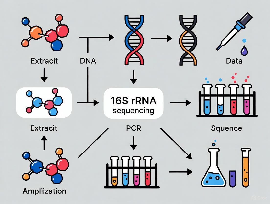
The standard 16S rRNA gene sequencing workflow comprises four critical stages: sample collection and preservation, DNA extraction, target amplification, and sequencing/library preparation. Each stage introduces specific considerations that can significantly impact downstream results and taxonomic classification accuracy. The fundamental workflow can be visualized as a sequential process with key decision points at each stage.
Figure 1: Essential 16S rRNA Gene Sequencing Workflow. This diagram outlines the core sequential steps and critical decision points in a standard 16S rRNA sequencing pipeline, from sample collection through data analysis.
Recent advancements have particularly focused on overcoming the limitations of short-read sequencing technologies. Traditional Sanger sequencing and Illumina-based approaches typically target partial 16S rRNA gene regions (e.g., V3-V4 or V4), which lack the discriminative power for reliable species-level identification [27] [15]. In contrast, third-generation sequencing platforms like Oxford Nanopore Technologies enable full-length 16S rRNA gene sequencing, spanning the V1-V9 regions, which provides significantly enhanced taxonomic resolution [5] [27]. This comprehensive approach is particularly valuable for clinical diagnostics, where species-level identification can directly impact patient management and antibiotic treatment decisions [29] [15].
Sample Collection & Preservation
Proper sample collection and preservation are critical first steps in ensuring accurate microbial community representation. Collection protocols must be tailored to specific sample types, while maintaining consistent sterilization and preservation conditions across all samples to minimize technical variability.
Sample-Type Specific Considerations
Human-Derived Samples: For fecal samples, collection should occur immediately before freezing at -20°C or -80°C to preserve microbial integrity [12]. Swab samples from skin or mucosal surfaces require sterile collection containers to prevent environmental contamination [12]. Clinical samples from sterile sites (e.g., tissue, cerebrospinal fluid, joint fluid) should be collected in sterile containers and processed rapidly, ideally with addition of preservation buffers if immediate freezing is not possible [30].
Environmental Samples: Soil and water samples require specific collection methodologies. Environmental water samples may need immediate filtration to concentrate biomass, while soil samples should be collected using sterile corers and transferred to sterile containers [5]. The ZymoBIOMICS DNA Miniprep Kit is recommended for environmental water samples, while the QIAGEN DNeasy PowerMax Soil Kit is optimal for soil samples [5].
Preservation Parameters
Immediate freezing at -20°C or -80°C is the gold standard for sample preservation [12]. When immediate freezing is not feasible, temporary storage at 4°C for up to 24 hours is acceptable, though preservation buffers can extend this window to several days [12]. Multiple freeze-thaw cycles should be strictly avoided, as they degrade DNA quality and alter microbial community representations [12]. For this reason, aliquoting samples prior to initial freezing is strongly recommended.
Table 1: Sample Collection and Preservation Guidelines by Sample Type
| Sample Type | Recommended Collection Method | Preservation Conditions | Special Considerations |
|---|---|---|---|
| Fecal | Sterile collection container | Immediate freezing at -80°C | Aliquot before freezing; avoid freeze-thaw cycles [12] |
| Tissue/Biopsy | Sterile surgical collection | Snap freezing in liquid nitrogen | Homogenize with lysis buffer before DNA extraction [30] |
| Swab | Sterile swab in transport medium | -20°C for short-term; -80°C for long-term | Low biomass samples prone to contamination [12] |
| Environmental Water | Filtration through sterile membranes | Freeze filters at -80°C | ZymoBIOMICS DNA Miniprep Kit recommended [5] |
| Soil | Sterile coring device | Freeze at -80°C | QIAGEN DNeasy PowerMax Soil Kit recommended [5] |
DNA Extraction Protocols
DNA extraction represents a crucial step where biases can be introduced, significantly impacting downstream microbial community analyses. The optimal extraction method must effectively lyse diverse bacterial cell types while yielding high-quality, inhibitor-free DNA suitable for amplification.
Extraction Methodology Selection
The choice of DNA extraction method should be guided by sample type and bacterial community characteristics. For complex samples containing Gram-positive bacteria, protocols incorporating enhanced lysis steps are essential. A modified DNeasy tissue kit (Qiagen) protocol for Gram-positive bacteria includes an initial achromopeptidase incubation (1 hour at 37°C) to ensure effective lysis of resistant cell walls [8]. This is followed by proteinase K (40 μl) and ATL buffer (180 μl) incubation at 55°C for 1 hour, with a final lysis step using AL buffer (200 μl) at 70°C for 10 minutes [8].
For clinical samples, mechanical lysis through bead beating is often necessary for efficient cell disruption. The AusDiagnostics MT-Prep system, used in conjunction with Lysing Matrix E tubes and a TissueLyser (50 oscillations/second for 2 minutes), provides effective homogenization for tissue samples [30]. Pre-processing of tissue samples with Tissue Lysis Buffer ATL and proteinase K for 2 hours at 56°C before bead-beating further enhances DNA yield [30].
Extraction Kits by Sample Type
Commercial extraction kits optimized for specific sample types can significantly improve DNA yield and quality. For stool samples, the QIAamp PowerFecal DNA Kit effectively extracts microbiome DNA, while the QIAGEN Genomic-tip 20/G provides a balanced extraction of both host and microbiome DNA [5]. The MagNA Pure 96 DNA Viral NA small volume Kit with the Pathogen Universal 200 protocol has been successfully implemented for clinical samples like cerebrospinal fluid, plasma, and abscess materials [15].
Table 2: DNA Extraction Methods and Their Applications
| Extraction Method/Kit | Sample Type Applications | Key Features | Protocol Modifications |
|---|---|---|---|
| DNeasy Tissue Kit (Qiagen) | Mucus, water filters, Gram-positive bacteria | Effective for diverse bacterial types | Achromopeptidase incubation (1h, 37°C); proteinase K + ATL buffer (55°C, 1h); AL buffer (70°C, 10min) [8] |
| QIAamp PowerFecal Pro DNA Kit | Stool, gut microbiome samples | Optimized for complex microbiomes | Bead-beating step enhances lysis efficiency [31] |
| AusDiagnostics MT-Prep | Clinical tissues, sterile fluids | Integrated system for clinical samples | Pre-processing with Tissue Lysis Buffer ATL + proteinase K (56°C, 2h); bead-beating with Lysing Matrix E [30] |
| MagNA Pure 96 DNA Viral NA | CSF, plasma, abscess, biopsy | Automated extraction for clinical diagnostics | Pathogen Universal 200 protocol; elution in 100μl volume [15] |
Target Amplification Strategies
Amplification of the 16S rRNA gene through polymerase chain reaction (PCR) requires careful optimization of primer selection and cycling conditions to minimize biases and maintain taxonomic representation.
Primer Selection and Region Choice
The selection of target regions within the 16S rRNA gene significantly influences taxonomic resolution. Full-length 16S rRNA gene amplification (V1-V9 regions, ~1.5 kb) using primers such as 16SV1-V9F (5'-TTT CTG TTG GTG CTG ATA TTG CAG RGT TYG ATY MTG GCT CAG-3') and 16SV1-V9R (5'-ACT TGC CTG TCG CTC TAT CTT CCG GYT ACC TTG TTA CGA CTT-3') provides maximum discriminative power for species-level identification [15]. For specific applications targeting hypervariable regions, primer sets such as Pro341F (5'-CCTA CGGGNBGCASCAG-3') and Pro805R (5'-GACTACNVGGGT ATCTAATCC-3') effectively amplify the V3-V4 regions [8].
Recent comparative studies demonstrate that full-length 16S rRNA gene sequencing significantly enhances species-level resolution compared to partial gene approaches. Nanopore full-length 16S rRNA sequencing identified specific bacterial biomarkers for colorectal cancer, including Parvimonas micra, Fusobacterium nucleatum, and Peptostreptococcus anaerobius, which were less reliably detected with Illumina V3-V4 sequencing [27].
PCR Optimization and Quality Control
PCR amplification should utilize high-fidelity DNA polymerases to minimize amplification errors. The iProof High-Fidelity polymerase (Bio-Rad) has been successfully implemented with the following cycling conditions: initial denaturation at 95°C for 3 minutes, followed by 35 cycles of 95°C for 30 seconds, 55°C for 30 seconds, 72°C for 30 seconds, and a final extension at 72°C for 5 minutes [8]. For full-length 16S rRNA amplification, the LongAmp Taq 2x MasterMix provides efficient amplification of long amplicons with conditions including 95°C for 2 minutes, 25 cycles of 95°C for 15 seconds, 55°C for 30 seconds, and 65°C for 75 seconds, followed by a final extension at 65°C for 10 minutes [15].
Innovative approaches like micelle-based PCR (micPCR) address common amplification artifacts by compartmentalizing individual template molecules, preventing chimera formation and PCR competition [15]. This method incorporates an internal calibrator (Synechococcus 16S rRNA gene copies) to enable absolute quantification and correct for background DNA contamination [15].
Post-amplification, quality assessment through agarose gel electrophoresis confirms amplicon size and purity, while quantification using fluorometric methods (e.g., Qubit dsDNA HS Assay) provides accurate DNA concentration measurements for downstream sequencing [8].
Sequencing & Library Preparation
Library preparation and sequencing platform selection critically influence data quality, turnaround time, and analytical capabilities. The emergence of long-read sequencing technologies has transformed the 16S rRNA sequencing landscape by enabling real-time, full-length analysis.
Library Preparation Methods
For Oxford Nanopore sequencing, the 16S Barcoding Kit 24 enables multiplexing of up to 24 samples in a single sequencing run, incorporating both amplification and barcoding steps [5]. The kit utilizes PCR to amplify the entire ~1.5 kb 16S rRNA gene from extracted gDNA with barcoded primers, followed by sequencing adapter addition [5]. For ligation-based approaches without amplification, the SQK-SLK109 protocol can be adapted for 16S sequencing with additional reagents from New England Biolabs (Cat. E7564, M0367, and E6056S) [29].
A high-throughput full-length 16S sequencing protocol developed for synthetic microbial communities demonstrates the efficiency of ONT ligation sequencing, achieving accurate community composition measurements with faster turnaround times compared to Illumina MiSeq [28]. This method processes 440 samples efficiently while maintaining precision across replicates, making it suitable for large-scale microbiome studies.
Sequencing Platforms and Parameters
Oxford Nanopore sequencing using MinION Flow Cells with the high accuracy (HAC) basecaller typically runs for 24-72 hours, depending on microbial sample complexity [5]. For rapid clinical diagnostics, Flongle Flow Cells provide a cost-effective solution for individual samples, reducing time to results to approximately 24 hours [15]. Sequencing settings typically include super-accurate basecalling, minimum qscore of 10, and read length filtering (200-500 bases for partial regions; 1,000-1,800 bases for full-length 16S) [29] [31].
The integration of PhiX Control library (approximately 15%) with the amplicon library serves as a sequencing quality control [8]. For flow cells not run at full capacity, the Flow Cell Wash Kit enables reuse, significantly reducing per-sample sequencing costs [5].
Table 3: Sequencing Platform Comparison for 16S rRNA Gene Sequencing
| Parameter | Illumina MiSeq | Oxford Nanopore MinION |
|---|---|---|
| Read Length | 300 bp (partial 16S regions) | Full-length 16S (~1,500 bp) [28] |
| Target Regions | Typically V3-V4 or V4 | V1-V9 (full gene) [5] |
| Time to Results | 2-3 days (batch processing) | 24-72 hours; 24h for Flongle [15] |
| Taxonomic Resolution | Genus-level | Species-level [27] |
| Library Preparation | Multi-step, prolonged [28] | Streamlined workflow [28] |
| Clinical Utility | Limited by turnaround time | Enhanced by rapid diagnostics [29] |
The Scientist's Toolkit
Implementing a robust 16S rRNA sequencing workflow requires specific reagents, kits, and instrumentation optimized for each procedural step. The following table details essential solutions for establishing a reliable laboratory pipeline.
Table 4: Essential Research Reagent Solutions for 16S rRNA Sequencing
| Product/Kit | Manufacturer | Application | Key Features |
|---|---|---|---|
| DNeasy PowerMax Soil Kit | QIAGEN | DNA extraction from soil | Effective for difficult-to-lyse environmental organisms [5] |
| QIAamp PowerFecal DNA Kit | QIAGEN | Stool DNA extraction | Optimized for complex gut microbiomes [5] |
| 16S Barcoding Kit 24 | Oxford Nanopore | Library preparation | Multiplexes 24 samples; includes barcoded primers [5] |
| ZymoBIOMICS Microbial Community Standards | Zymo Research | Process controls | Characterized mock communities for quality control [31] |
| iProof High-Fidelity DNA Polymerase | Bio-Rad | 16S rRNA amplification | High-fidelity PCR reducing amplification errors [8] |
| LongAmp Taq 2x MasterMix | New England Biolabs | Full-length 16S amplification | Efficient amplification of ~1.5 kb 16S gene [15] |
| SQK-PCB114.24 Barcodes | Oxford Nanopore | Library barcoding | Enables sample multiplexing on Flongle/MiniON [15] |
The comprehensive workflow outlined in this application note provides researchers and clinical scientists with a robust framework for implementing 16S rRNA gene sequencing in both research and diagnostic contexts. The integration of full-length 16S rRNA sequencing through long-read technologies represents a significant advancement over traditional short-read approaches, enabling species-level taxonomic resolution that is critical for biomarker discovery, clinical diagnostics, and therapeutic development.
As sequencing technologies continue to evolve, standardization of protocols and implementation of rigorous quality control measures will be essential for generating reproducible, clinically actionable data. The methodologies detailed herein serve as a foundation for advancing microbial community analyses across diverse fields, from environmental microbiology to personalized medicine. By adhering to these optimized workflows and maintaining awareness of emerging technological improvements, researchers can maximize the analytical power of 16S rRNA sequencing for both fundamental discovery and applied diagnostic applications.
Optimized Protocols for 16S rRNA Sample Preparation Across Diverse Specimens
Within the framework of 16S rRNA sequencing sample preparation research, the initial steps of sample collection and preservation are paramount. The integrity of nucleic acids directly dictates the success and accuracy of all subsequent sequencing data, influencing downstream taxonomic classification and diversity analyses [16] [32]. This application note provides detailed protocols and key considerations for ensuring nucleic acid integrity from sample acquisition to library preparation, specifically tailored for microbiome studies utilizing 16S rRNA gene sequencing.
The goal is to furnish researchers and drug development professionals with standardized methodologies that minimize bias, preserve true microbial community structure, and ensure the reliability of sequencing results for both clinical diagnostics and research applications.
Critical Considerations for Sample Collection
The choice of collection method is highly dependent on the sample origin, as different anatomical sites and sample matrices present unique challenges for microbial biomass and integrity.
Sample Type-Specific Protocols
- Oropharyngeal Swabs: For profiling the human oropharyngeal microbiome, systematic sampling is recommended. Swabs should first be applied to the teeth, tongue, and buccal mucosa before insertion into the pharynx to ensure comprehensive collection [16]. The use of sterile swabs is critical to avoid external contamination.
- Fecal Samples: The human gut microbiome is a complex matrix with varying consistency and microbial load. Standardization of the sample amount is essential. Recent studies highlight the utility of stool preprocessing devices (SPD) to homogenize the sample prior to DNA extraction, which significantly improves DNA yield, standardization, and the recovery of Gram-positive bacteria with tough cell walls [32].
Universal Collection Principles
- Use of Preservation Buffers: Immediately upon collection, samples should be transferred into an appropriate DNA/RNA shielding buffer [16]. These buffers are designed to stabilize nucleic acids by inhibiting nuclease activity and preventing the overgrowth of any single microbial population, thereby preserving the in vivo microbial community structure.
- Minimizing Time to Preservation: The interval between sample collection and immersion in preservation buffer should be minimized to reduce the risk of nucleic acid degradation and shifts in microbial composition.
Sample Preservation and Storage Workflow
The following diagram illustrates the critical decision points and workflow for proper sample handling from collection to analysis.
DNA Extraction and Quality Control
The DNA extraction protocol must be robust and efficient to lyse a wide range of bacterial cells while yielding high-quality, high-molecular-weight DNA.
Recommended Extraction Methodology
Based on comparative studies, the following method is recommended for gut microbiome samples:
- Protocol: Combine a stool preprocessing device (SPD) with the DNeasy PowerLyzer PowerSoil kit (QIAGEN) [32]. This protocol, referred to as S-DQ, has been shown to provide an optimal balance of DNA yield, fragment size, and purity.
- Key Step: Incorporate a rigorous bead-beating step using a PowerLyzer instrument. This is crucial for the effective lysis of Gram-positive bacteria, which have thick peptidoglycan cell walls, thereby reducing community composition bias [32].
For oropharyngeal swabs, the Quick-DNA HMW MagBead kit (Zymo Research) has been successfully used in conjunction with swabs stored in shielding buffer [16].
Quality Control Assessment
Post-extraction, DNA quality must be verified using multiple metrics, as summarized in the table below.
Table 1: Quality Control Metrics for Extracted Genomic DNA
| Parameter | Target Value | Assessment Method | Significance for 16S Sequencing |
|---|---|---|---|
| DNA Concentration | > 5 ng/µL [32] | Fluorometry (e.g., Qubit) | Ensures sufficient template for library preparation. |
| DNA Purity (A260/280) | ~1.8 [32] | Spectrophotometry (e.g., NanoDrop) | A low ratio indicates protein contamination; a high ratio suggests RNA residue. |
| DNA Fragment Size | > 10,000 bp [32] | Electrophoresis (e.g., TapeStation) | Indicates high-molecular-weight DNA, suitable for full-length amplicon sequencing. |
The Scientist's Toolkit: Research Reagent Solutions
Table 2: Essential Materials and Reagents for Sample Collection, Preservation, and DNA Extraction
| Item | Function | Example Product & Manufacturer |
|---|---|---|
| DNA/RNA Shielding Buffer | Stabilizes nucleic acids immediately after collection, inhibiting nucleases and microbial growth. | DNA/RNA Shield (Zymo Research) [16] |
| Sterile Swabs | Collection of samples from mucosal surfaces like the oropharynx. | Various manufacturers [16] |
| Stool Preprocessing Device (SPD) | Standardizes and homogenizes fecal samples prior to DNA extraction, improving yield and reproducibility. | SPD (bioMérieux) [32] |
| Bead-Beating DNA Extraction Kit | Efficiently lyses Gram-positive and Gram-negative bacteria; purifies nucleic acids. | DNeasy PowerLyzer PowerSoil Kit (QIAGEN) [32] |
| Internal Spike-In Controls | Distinguishes true low-abundance taxa from contamination; enables absolute quantification [31] [33]. | ZymoBIOMICS Spike-in Control (Zymo Research) [31] |
Managing Contamination and Bias
A critical aspect of preserving nucleic acid integrity is managing technical artifacts that can distort true microbial profiles.
Contamination Mitigation Strategy
Microbial DNA contamination from reagents and kits is a major challenge, particularly in low-biomass samples. The following workflow, adapted from modern clinical microbiology practices, outlines a robust strategy for identifying and filtering contamination.
The criteria for filtering based on the Frequency Threshold (FT) are [33]:
- Accept: Any bacterium with an abundance higher than the top five abundant contaminants.
- Review: Bacteria present at frequencies between 20% and 100% of the FT, but only if absent from all negative controls.
- Reject: Bacteria present at frequencies below 20% of the FT.
Primer Selection for Amplification
The choice of PCR primers for 16S rRNA gene amplification is a significant source of bias. Studies on oropharyngeal samples demonstrate that degenerate primers (e.g., the 27F-II variant: 5’- AGRGTTTGATCMTGGCTCAG -3') yield significantly higher alpha diversity and a more balanced taxonomic profile compared to non-degenerate or less degenerate standard primers [16]. These primers, which incorporate nucleotide ambiguity codes (like 'R' for A/G and 'M' for A/C), improve amplification inclusivity across a broader range of bacterial taxa, reducing taxonomic dropout.
Rigorous sample collection and preservation protocols are the foundational pillars of robust 16S rRNA sequencing research. The adoption of standardized methods—including immediate sample preservation in specialized buffers, the use of homogenization devices for complex matrices, optimized bead-beating DNA extraction, and systematic contamination tracking—is critical for generating reliable and reproducible microbiome data. By implementing the detailed protocols and considerations outlined in this application note, researchers can significantly enhance nucleic acid integrity from the very first step, thereby ensuring the fidelity of downstream taxonomic and biomarker discoveries in both research and drug development contexts.
Within the framework of 16S rRNA sequencing sample preparation research, the selection of an appropriate DNA extraction method is a critical determinant of experimental success. The DNA extraction process introduces significant variability in microbial community profiling, impacting downstream analyses including diversity metrics and taxonomic classification [34]. This application note provides a structured guide to selecting and optimizing DNA extraction protocols tailored to specific sample types, with a focus on 16S rRNA sequencing for microbiome studies.
The Impact of DNA Extraction on 16S rRNA Sequencing
DNA extraction methodology directly influences multiple aspects of 16S rRNA sequencing data. The process encompasses bacterial cell lysis, DNA purification, and removal of contaminants, each step potentially introducing bias. Specifically, the lysis efficiency varies considerably between Gram-positive and Gram-negative bacteria due to differences in cell wall structure. Gram-positive bacteria, with their thick peptidoglycan layer, often require vigorous mechanical lysis (bead-beating) for optimal DNA recovery, whereas Gram-negative bacteria are more susceptible to chemical and enzymatic lysis [34] [35].
Furthermore, the purity and yield of the extracted DNA affect PCR amplification during library preparation. The presence of inhibitors or excessive host DNA can lead to amplification failure or skewed representation of microbial communities [36]. Studies have demonstrated that the choice of extraction kit can affect the observed microbial diversity, with protocols incorporating mechanical lysis generally recovering a greater proportion of Gram-positive bacteria and thus providing a more representative community profile [34] [32].
Sample Type-Specific Kit Selection and Performance Data
The optimal DNA extraction strategy is highly dependent on the sample type, primarily due to variations in microbial load, sample biomass, and the presence of PCR inhibitors. The following sections and tables summarize key performance metrics across different sample categories.
High-Biomass Samples (e.g., Stool)
For high-biomass samples like stool, multiple kits perform reliably. A comparative study of four commercial kits on fecal samples found that while DNA quantity and quality varied, the resulting microbiota profiles showed similar diversity and compositional patterns [34].
Table 1: Performance of DNA Extraction Kits for High-Biomass Stool Samples
| Kit Name | Lysis Method | DNA Binding Method | Performance Notes |
|---|---|---|---|
| QIAamp PowerFecal Pro DNA Kit (QIAGEN) [34] | Mechanical & Chemical | Silica Membrane | Robust performance; includes bead-beating for efficient lysis. |
| Macherey NucleoSpin Soil Kit (MACHEREY-NAGEL) [34] | Mechanical & Chemical | Silica Membrane | Effective for diverse bacterial communities. |
| PureLink Microbiome DNA Purification Kit (Thermo Fisher) [37] | Heat, Chemical & Mechanical (Triple-Lysis) | Spin Column | Recovers 2–5 times more DNA than some competitors; effective inhibitor removal. |
| DNeasy PowerLyzer PowerSoil (QIAGEN) [32] | Mechanical & Chemical | Silica Membrane | Shows high DNA yield and purity; performance further improved with a stool preprocessing device (SPD). |
Low-Biomass Samples (e.g., BAL, Sputum, Swabs)
Low-biomass samples present a greater challenge, often yielding low DNA concentrations and being more susceptible to contamination. None of the four kits evaluated in one study (QIAamp PowerFecal Pro, NucleoSpin Soil, NucleoSpin Tissue, and MagnaPure LC DNA isolation kit III) were deemed sufficiently sensitive for optimal performance with low-biomass samples such as bronchoalveolar lavage (BAL) and sputum [34]. For these samples, specialized kits that include host DNA depletion are recommended.
Table 2: Performance of DNA Extraction Kits for Low-Biomass and Host-Rich Samples
| Kit Name | Key Feature | Sample Types | Performance Notes |
|---|---|---|---|
| QIAamp DNA Microbiome Kit (QIAGEN) [36] | Integrated Host DNA Depletion | Swabs, Body Fluids | Effectively removes host DNA (e.g., <5% human reads in buccal swabs vs. >90% with non-depleting kits). |
| PureLink Microbiome DNA Purification Kit (Thermo Fisher) [37] | Versatile for multiple types | Urine, Saliva, Swabs | Uses a triple-lysis approach for durable microorganisms. |
Challenging and Specialized Samples
The physical and chemical properties of some samples require tailored extraction approaches.
- Gram-Positive Bacteria: Kits employing mechanical lysis (bead-beating) are essential. For instance, in an extraction from Bacillus subtilis (a Gram-positive bacterium), the Qiagen Blood & Cell Culture DNA Midi Kit and the BIOG kit yielded high DNA concentrations (~1500 ng/μL) and good purity (A260/A280 ~1.8), significantly outperforming a kit without optimized lysis (488 ng/μL) [35].
- Plant Material: Samples rich in polysaccharides and polyphenols (e.g., tea leaves) require kits with special additives to remove these contaminants, aiming for ideal purity ratios of A260/A280 = 1.8-2.0 and A260/A230 > 2.0 [38].
- Cell-Free DNA: Isolation from plasma or serum requires kits designed for low abundance targets, often using magnetic beads for efficient capture from large volume samples [37].
Detailed Experimental Protocols
Protocol: DNA Extraction from Stool Using a Bead-Beating Kit
This protocol is adapted from the methods used with the QIAamp PowerFecal Pro DNA Kit and provides a general framework for manual extraction of bacterial DNA from stool samples [34].
Research Reagent Solutions:
- Lysis Buffer: Contains salts and detergents to begin disrupting cells.
- PowerBead Pro Tubes: Tubes containing a mixture of ceramic beads for mechanical lysis.
- Binding Buffer: Facilitates the attachment of DNA to the silica membrane.
- Wash Buffers: Typically ethanol-based, used to remove salts, proteins, and other impurities.
- Elution Buffer: Low-salt buffer (e.g., Tris-HCl or TE buffer) to release purified DNA from the membrane.
Procedure:
- Sample Preparation: Weigh approximately 200 mg of stool and suspend it in 100 μL of PBS. Alternatively, use the specific buffer provided in the kit.
- Mechanical Lysis:
- Transfer the entire sample mixture into a PowerBead Pro Tube.
- Securely close the tube and vortex at high speed for 5-10 minutes to ensure thorough homogenization and cell disruption.
- Briefly centrifuge the tube to collect the contents at the bottom.
- Binding: Add the recommended volume of binding buffer to the lysate and mix. Transfer the mixture to an MB Spin Column and centrifuge. The DNA binds to the silica membrane while contaminants pass through.
- Washing:
- Add wash buffer 1 to the column, centrifuge, and discard the flow-through.
- Add wash buffer 2 (often containing ethanol), centrifuge, and discard the flow-through. This step may be repeated.
- Perform a final "empty" spin to remove residual ethanol.
- Elution:
- Transfer the column to a clean 1.5 mL microcentrifuge tube.
- Add 50-100 μL of Elution Buffer (C6 buffer) directly onto the center of the membrane.
- Incubate at room temperature for 1-5 minutes, then centrifuge to elute the purified DNA.
- Storage: Store the extracted DNA at -80°C until ready for downstream application.
Protocol: DNA Extraction with Host DNA Depletion
This protocol outlines the procedure for the QIAamp DNA Microbiome Kit, designed for samples like buccal swabs where host DNA significantly outweighs microbial DNA [36].
Procedure:
- Host Cell Lysis: The sample is treated with a gentle lysis buffer that selectively ruptures human/animal cells while leaving bacterial cells intact.
- Host DNA Digestion: The released host DNA is enzymatically degraded using a DNase.
- Microbial Cell Lysis: Bacterial cells are lysed using an optimized combination of mechanical and chemical lysis to minimize bias against tough-to-lyse bacteria.
- DNA Binding and Purification: The released bacterial DNA is purified using Ultra Clean Production (UCP) spin columns and standard wash steps to remove contaminants.
- Elution: The purified microbial DNA is eluted in a low-salt elution buffer.
The following workflow diagram illustrates the key steps and decision points in selecting a DNA extraction method for 16S rRNA sequencing.
Essential Research Reagent Solutions
The following table details key reagents and their critical functions in the DNA extraction workflow for microbiome studies.
Table 3: Essential Research Reagent Solutions for Bacterial DNA Extraction
| Reagent / Material | Function | Application Notes |
|---|---|---|
| Bead Tubes (Ceramic/Silica) [34] [32] | Mechanical cell disruption (bead-beating) for tough cell walls. | Critical for lysing Gram-positive bacteria; bead material and size can influence efficiency. |
| Proteinase K [34] | Enzymatic digestion of proteins and disruption of cellular structures. | Used in enzymatic lysis protocols; often combined with heat treatment (e.g., 56°C). |
| Silica Membrane Columns [34] [36] | Selective binding and purification of DNA from lysates. | The basis for many commercial kits; allows for washing away impurities. |
| Magnetic Beads [34] [37] | High-throughput DNA binding and purification using magnetic separation. | Common in automated systems; efficient for processing large sample volumes. |
| Inhibitor Removal Buffers [37] | Precipitation or neutralization of common PCR inhibitors (e.g., humic acids, bile salts). | Essential for complex samples like stool, soil, and plant material. |
| Host Depletion Enzymes [36] | Selective digestion of host (e.g., human) genomic DNA after gentle lysis of host cells. | Vital for low-biomass samples where host DNA can dominate sequencing reads. |
The selection of a DNA extraction kit must be a deliberate decision tailored to the specific sample type and research objectives in 16S rRNA sequencing studies. Key considerations include the sample's biomass, the bacterial community structure (notably the abundance of Gram-positive organisms), and the level of contaminating host DNA. Protocols that incorporate mechanical lysis, such as bead-beating, are generally recommended for comprehensive lysis of diverse bacterial communities. Furthermore, for host-rich samples, kits with integrated host DNA depletion are invaluable for increasing the sensitivity and cost-effectiveness of sequencing. By aligning the extraction methodology with the sample's inherent properties, researchers can minimize bias and generate more reliable and reproducible microbiome data.
In 16S rRNA gene sequencing, the selection of PCR primers is a foundational step that directly determines the accuracy and reliability of subsequent microbiome analysis. The 16S rRNA gene contains nine hypervariable regions (V1-V9), flanked by conserved sequences, which are used for primer design [39] [12]. Coverage refers to the fraction of bacterial sequences in a sample that a primer pair can successfully target and amplify, while specificity indicates its ability to amplify only the intended 16S rRNA sequences without off-target binding [40] [41]. Achieving an optimal balance between these two factors is critical, as biases introduced during primer selection can lead to significant inaccuracies in taxonomic abundance and diversity estimates [39] [42]. This application note details standardized protocols and decision frameworks to guide researchers in selecting and validating 16S rRNA primers, thereby minimizing bias within 16S rRNA sequencing sample preparation workflows.
Primer Performance Across Variable Regions
The choice of which hypervariable region(s) to amplify is a primary source of variability in 16S rRNA sequencing outcomes. Different variable regions exhibit substantial differences in their ability to detect and accurately represent specific bacterial taxa.
Table 1: In Silico Coverage of Different 16S rRNA Primer Pairs Against a Reference Database (eHOMD)
| Target Region | Forward Primer | Reverse Primer | Approximate Amplicon Size (bp) | Percentage of Original Input Sequences Detected |
|---|---|---|---|---|
| V1-V2 | AGAGTTTGATYMTGGCTCAG | TGCTGCCTCCCGTAGRAGT | 311 | >90% |
| V3-V4 | CCTACGGGNGGCWGCAG | GACTACHVGGGTATCTAATCC | 444 | >90% |
| V4-V5 | GTGYCAGCMGCCGCGGTAA | CCGYCAATTYMTTTRAGTTT | 411 | >90% |
| V1-V3 | TNANACATGCAAGTCGRRCG | WTTACCGCGGCTGCTGG | 450 | <70% |
| V6-V8 | CAACGCGAAGAACCTTACC | GACGGGCGGTGWGTRCA | 424 | <70% |
Comparative studies consistently show that primer choice significantly influences the observed microbial composition, with clustering in multidimensional scaling plots often being more driven by the primer pair used than by the biological sample source itself [39]. For instance, in human gut microbiome studies, the V1-V2 and V3-V4 regions are widely used, but they can yield different profiles; the V3-V4 primer set has been reported to detect higher relative levels of Akkermansia and Bifidobacterium compared to the V1-V2 set, even though follow-up qPCR validation suggested that the V1-V2 data might be closer to the actual abundance for Akkermansia [43]. Furthermore, some primer pairs systematically miss specific phyla. For example, the primer pair 515F-944R (targeting V4-V5) was found to miss Bacteroidetes, and no single primer pair can capture the full spectrum of microbial diversity present in a complex sample [39].
Experimental Protocol for Primer Selection and Validation
A robust primer selection and validation protocol is essential for generating reliable 16S rRNA sequencing data. The following workflow provides a systematic approach.
Figure 1: A workflow for the systematic selection and validation of 16S rRNA gene sequencing primers. Key considerations at each stage are highlighted.
In Silico Evaluation of Primer Candidates
Purpose: To computationally predict the coverage and specificity of candidate primer pairs before costly wet-lab experiments. Procedure:
- Compile Primer Sequences: Gather a list of candidate primer pairs from the literature (e.g., [44] [41]).
- Select Reference Database: Obtain full-length 16S rRNA gene sequences from a curated database such as SILVA, GreenGenes, or the Human Oral Microbiome Database (HOMD) for in silico simulation [44] [42].
- Generate In Silico Amplicons: Use bioinformatic tools (e.g., Seqkit, TestPrime) to trim the full-length reference sequences to the regions defined by each candidate primer pair [44] [42].
- Calculate Coverage and Specificity:
- Coverage: Determine the percentage of reference sequences that are successfully amplified by the primer pair. A high-coverage primer should amplify >90% of sequences for the phyla of interest [44].
- Specificity: Check for potential off-target amplification, including against the host genome (e.g., human mitochondrial DNA), which is a critical issue for biopsy samples [41].
Wet-Lab Validation with Controls
Purpose: To empirically confirm the performance of primers selected from the in silico analysis. Procedure:
- DNA Extraction: Extract genomic DNA from your sample types using a standardized, bead-beating included method to ensure efficient lysis of all cell types [43] [45].
- PCR Amplification:
- Use a high-fidelity DNA polymerase to minimize PCR errors [45].
- Primer Mixture: For regions with known biases, consider using a modified primer mixture. For example, to recover Fusobacteriota missed by a standard V1-V2 primer, include a specific forward primer (68F_M) in the reaction mix [41].
- PCR Setup: Evidence suggests that conducting a single PCR reaction per sample, rather than pooling multiple technical replicates, does not significantly impact outcomes and saves reagents and time [45].
- Mastermix: Using a commercially available premixed mastermix is acceptable and does not introduce significant bias compared to manually prepared mastermix, thereby streamlining the protocol [45].
- Essential Controls:
- Mock Microbial Community: Always include a commercially available mock community (e.g., ZymoBIOMICS standards) with a known composition. This positive control is vital for assessing amplification bias, accuracy, and detecting reagent contamination [39] [45].
- Negative Controls: Include a non-template control (NTC) with PCR-grade water to identify any contamination from reagents or the environment [45].
- Sample Extraction Control: For low-biomass samples, include a control that undergoes the extraction process without any sample to monitor kit-borne contaminants [45].
Bioinformatic Processing and Data Interpretation
Purpose: To process sequencing data and evaluate the performance of the tested primers. Procedure:
- Sequence Processing: Use a pipeline like QIIME2 or DADA2 for denoising, paired-end read merging, and chimera removal. This generates amplicon sequence variants (ASVs) [43] [46].
- Taxonomic Assignment: Assign taxonomy to ASVs using a naive Bayes classifier trained on a reference database (e.g., GreenGenes, SILVA) tailored to the amplified variable region [44] [43].
- Performance Analysis:
- For Mock Communities: Compare the observed composition of the mock community to its known composition. Calculate the rate of false positives, false negatives, and the accuracy of relative abundance estimates [39].
- For Biological Samples: Analyze alpha and beta diversity metrics. Compare the taxonomic profiles generated by different primer pairs, focusing on the detection of key taxa relevant to your research question [43] [41].
The Scientist's Toolkit: Research Reagent Solutions
Table 2: Essential Reagents and Materials for 16S rRNA Primer Evaluation
| Item | Function / Rationale | Examples / Considerations |
|---|---|---|
| High-Fidelity DNA Polymerase | Reduces PCR errors during amplification of complex microbial DNA. | Q5 Hot Start High-Fidelity Mastermix (NEB) [45]. |
| Mock Microbial Community | Validates primer accuracy and identifies amplification biases against a known standard. | ZymoBIOMICS Microbial Community Standard [45]. |
| Standardized DNA Extraction Kit | Ensures reproducible and unbiased lysis across all samples, including tough-to-lyse cells. | DNeasy PowerSoil Kit (QIAGEN); should include mechanical lysis [43] [45]. |
| Curated 16S rRNA Database | Provides reference sequences for in silico analysis and taxonomic classification. | SILVA, GreenGenes, Human Oral Microbiome Database (HOMD) [44] [42]. |
| Bioinformatic Pipelines | Processes raw sequencing data into denoised amplicon sequence variants (ASVs) for analysis. | QIIME2, DADA2 [43] [46]. |
Troubleshooting Common Primer-Related Issues
- Problem: Off-Target Amplification of Host DNA. A significant portion of sequences aligns to the host (e.g., human) genome, particularly in biopsy samples [41].
- Solution: Primers targeting the V1-V2 region have demonstrated a marked reduction in off-target human DNA amplification compared to the commonly used V4 primers. For esophageal, stomach, and duodenal biopsies, a modified V1-V2 primer set (V1-V2M) reduced human DNA alignment to nearly zero [41].
- Problem: Failure to Detect Specific Taxa. Known members of the microbiome are consistently absent from the data.
- Solution: Review in silico analysis for mismatches between your primer and the target taxon's 16S gene. If a critical taxon (e.g., Fusobacteriota) is not amplified due to a primer mismatch, consider using a primer mixture that includes a tailored primer for that group [41].
- Problem: Low Sequencing Depth or Poor Library Yield for Low-Biomass Samples.
- Solution: Optimize PCR cycle numbers to avoid excessive cycles that amplify background contamination. The use of a single, larger-volume PCR reaction is sufficient and improves efficiency [45]. Meticulously include and sequence negative controls to identify and subtract contaminating sequences.
The selection of 16S rRNA gene primers is a critical parameter that requires careful consideration of the trade-offs between coverage, specificity, and the specific research context. There is no single "perfect" universal primer pair. A rigorous, multi-stage validation protocol—incorporating in silico screening, wet-lab testing with mock communities and negative controls, and thoughtful bioinformatic analysis—is essential for generating robust and interpretable microbiome data. By adopting the systematic approach outlined in this application note, researchers can make informed decisions in primer design and selection, thereby minimizing bias and enhancing the reliability of their 16S rRNA sequencing results in drug development and basic research.
Library Preparation for Short-Read (Illumina) and Long-Read (Nanopore, PacBio) Platforms
Within 16S rRNA sequencing sample preparation research, a fundamental challenge lies in selecting and optimizing the library preparation protocol to match the sequencing platform with the specific biological question. The choice between short-read (Illumina) and long-read (Nanopore, PacBio) platforms dictates the experimental workflow, the region of the 16S rRNA gene that can be targeted, and ultimately, the taxonomic resolution achievable in the resulting microbial community data [47] [48]. This application note provides detailed methodologies and comparative data to guide researchers in executing robust library preparation for each major sequencing platform.
Platform Comparison and Selection
The performance of sequencing platforms varies significantly in output and taxonomic resolution, influenced by read length and accuracy. The table below summarizes key comparative metrics from recent studies.
Table 1: Quantitative comparison of sequencing platform performance in 16S rRNA gene sequencing
| Platform | Target Region | Average Read Length | Species-Level Classification Rate | Key Strengths | Noted Limitations |
|---|---|---|---|---|---|
| Illumina MiSeq | V3-V4 (~442 bp) | 442 ± 5 bp | 47% - 48% [47] | High output read counts; Q30+ accuracy [49] | Lower species-level resolution; primer/region bias [48] |
| PacBio Sequel II (HiFi) | Full-length (V1-V9, ~1,453 bp) | 1,453 ± 25 bp [47] | 63% [47] | High-fidelity (Q27) long reads; excellent species-level resolution [47] [50] | Higher initial instrument cost |
| ONT MinION (R9.4.1/R10.4.1) | Full-length (V1-V9, ~1,412 bp) | 1,412 ± 69 bp [47] | 76% [47] [27] | Real-time sequencing; rapid turnaround; low-cost device [49] [29] | Higher raw error rate requires specialized bioinformatics [47] [27] |
The selection of the target region is a critical determinant of taxonomic resolution. While short-read sequencing of the V3-V4 regions is often sufficient for genus-level classification [48] [50], multiple studies have demonstrated that full-length 16S rRNA gene sequencing with long-read platforms consistently enables higher species-level classification [47] [27] [5]. However, a significant challenge across all platforms is that many sequences classified at the species level are assigned ambiguous names like "uncultured_bacterium," which currently limits the immediate improvement in biological understanding [47].
Experimental Protocols
Universal Starting Material: DNA Extraction
The initial step for all platforms is the isolation of high-quality genomic DNA. The consistent use of the same extracted DNA across different platforms is essential for meaningful comparative studies [47]. Recommended kits are sample-specific:
- Stool samples: QIAamp PowerFecal DNA Kit [5] or DNeasy PowerSoil Kit [47].
- Soil samples: QIAGEN DNeasy PowerMax Soil Kit [5].
- Clinical samples (tissue, fluid): Bead-beating (e.g., with Lysing Matrix E tubes) followed by extraction with kits such as the QIAamp DNA/Blood Kit or EZ1&2 Virus Mini Kit [51] [30].
DNA should be quantified using a fluorometer (e.g., Qubit) and quality assessed by electrophoresis or Fragment Analyzer.
Platform-Specific Library Preparation Protocols
Illumina MiSeq (Short-Read) Protocol
This protocol targets the V3-V4 hypervariable regions.
- PCR Amplification:
- Primers: Use primers 341F and 785R as per Klindworth et al. (2013) [47].
- Protocol: Amplify microbial genomic DNA following the 16S Metagenomic Sequencing Library Preparation guide from Illumina. The reaction includes Illumina adapter overhangs.
- Index Ligation and Library Construction:
- Attach dual indices and sequencing adapters using the Nextera XT Index Kit [47].
- Library Quality Control:
- Verify the library's size and quality using a Bioanalyzer DNA 1000 chip [47].
Pacific Biosciences Sequel II (Long-Read) Protocol
This protocol amplifies the full-length 16S rRNA gene.
- PCR Amplification:
- Library Preparation:
- Quality Control:
- Assess the final library concentration and size distribution using a Qubit HS DNA Kit and a Fragment Analyzer [47].
Oxford Nanopore Technologies MinION (Long-Read) Protocol
This protocol also targets the full-length V1-V9 regions.
- PCR Amplification and Barcoding:
- Library Preparation:
- Purify the PCR product, quantify, and pool samples equimolarly.
- The prepared library includes the amplicons with attached barcodes and sequencing adapters [47].
- Sequencing:
Bioinformatic Analysis Workflows
The different error profiles of each platform necessitate tailored bioinformatics pipelines.
Table 2: Standardized bioinformatics pipelines for each sequencing platform
| Platform | Primary Data Type | Recommended Denoising/Clustering Tool | Typical Post-Processing Environment | Key Consideration |
|---|---|---|---|---|
| Illumina | Paired-end short reads | DADA2 (for ASVs) [47] | QIIME2 [47] | High accuracy allows for single-nucleotide resolution [49]. |
| PacBio HiFi | Long-read CCS reads | DADA2 (for ASVs) [47] | QIIME2 [47] | Circular Consensus Sequencing (CCS) generates high-fidelity (HiFi) reads suitable for DADA2 [47]. |
| ONT | Long-read single pass | Spaghetti (for OTUs) or Emu [47] [27] | EPI2ME wf-16s or QIIME2 [29] [5] | Higher error rate makes DADA2 denoising problematic; OTU clustering or tools like Emu are better suited [47] [27]. |
For taxonomic assignment, a Naïve Bayes classifier trained on the SILVA database is commonly used in QIIME2. The classifier should be customized for each platform by incorporating the specific primers and read length distributions used in the study [47].
The Scientist's Toolkit
Table 3: Essential research reagents and kits for 16S rRNA library preparation
| Item | Function | Example Products/Models |
|---|---|---|
| DNA Extraction Kits | Isolation of inhibitor-free microbial gDNA from complex samples. | QIAamp PowerFecal DNA Kit, DNeasy PowerSoil Kit, ZymoBIOMICS DNA Miniprep Kit [47] [5] [52] |
| High-Fidelity DNA Polymerase | Accurate amplification of the 16S rRNA gene target region with low error rate. | KAPA HiFi Hot Start DNA Polymerase [47] |
| Platform-Specific Library Prep Kits | Preparing amplicons for sequencing with platform-specific adapters. | Illumina: 16S Metagenomic Library Prep; PacBio: SMRTbell Express Template Prep Kit; ONT: 16S Barcoding Kit [47] [5] |
| Quantification & QC Instruments | Accurate quantification and quality assessment of nucleic acids. | Fluorometer (Qubit), Fragment Analyzer/Bioanalyzer [47] [48] |
| Sequencing Platforms | Generating sequence data. | Illumina MiSeq; PacBio Sequel II/IIe; ONT MinION/GridION [47] [48] |
| Bioinformatics Software | Data processing, denoising, taxonomic assignment, and diversity analysis. | QIIME2, EPI2ME wf-16s, DADA2, Emu, Spaghetti [47] [27] [5] |
Workflow Visualization
Targeting Hypervariable Regions vs. Full-Length 16S rRNA Gene Sequencing
The selection of amplification target is a critical initial step in 16S rRNA gene sequencing, fundamentally influencing the taxonomic resolution and data quality of microbiome studies. Researchers must choose between sequencing specific hypervariable regions (HRs) using short-read platforms or targeting the full-length gene with third-generation sequencing (TGS) technologies. This decision carries significant implications for phylogenetic resolution, cost-efficiency, and technical feasibility, particularly when working with challenging samples or limited DNA resources. The choice must be strategically aligned with the specific research objectives, whether they require broad microbial profiling or precise strain-level differentiation for therapeutic development [53] [54].
Within the context of 16S rRNA sequencing sample preparation research, this application note provides a structured comparison of these approaches. We present quantitative data on the resolving power of different hypervariable regions across distinct biological niches, detailed experimental protocols for both pathways, and a curated toolkit of essential reagents to guide researchers in making evidence-based methodological decisions.
Comparative Analysis of Sequencing Approaches
Performance Metrics Across Hypervariable Regions
Table 1: Taxonomic Resolution of Hypervariable Regions Across Sample Types
| Target Region | Sample Type | Recommended Use | Key Performance Findings | Primary Reference |
|---|---|---|---|---|
| V1-V3 | Skin Microbiome | Skin microbial ecology | Comparable resolution to full-length 16S for high-abundance bacteria at genus level [53]. | PMC11264597 |
| V1-V2 | Respiratory Sputum | Chronic respiratory disease | Highest sensitivity/specificity (AUC: 0.736); optimal for taxonomic identification in sputum [55]. | Sci Rep 13, 3974 (2023) |
| V3-V4 | General Microbiome | Standardized Illumina protocols | Common default; balances read length with Illumina sequencing chemistry [8]. | Bio-protocol.org |
| Full-Length (V1-V9) | Human Fecal Samples | Species-level biomarker discovery | Enables species-level identification; reveals clinically relevant CRC biomarkers [27]. | Sci Rep 15, 26486 (2025) |
| Full-Length (V1-V9) | Complex Bacterial Communities | Maximum phylogenetic resolution | Superior taxonomic resolution; enables strain-level differentiation for therapeutic development [54] [56]. | DDW Volume 26 – Issue 4 |
Technical Considerations for Method Selection
Full-length 16S rRNA gene sequencing via PacBio or Oxford Nanopore Technologies (ONT) provides the highest taxonomic resolution, enabling differentiation at the species and strain levels. This approach is particularly valuable for discovering precise bacterial biomarkers and developing targeted live biotherapeutics, as it leverages the complete discriminatory power of all nine variable regions [54] [27]. While traditionally associated with higher error rates, recent improvements in ONT chemistry (R10.4.1) and basecalling models (Dorado) have significantly enhanced accuracy, making species-level identification more reliable [27]. However, this method typically involves higher initial instrumentation costs and more complex data processing workflows.
Hypervariable region targeting remains a practical and cost-effective strategy, especially when using accessible Illumina platforms. The optimal hypervariable region varies significantly by sample type and research question. For instance, the V1-V3 region demonstrates performance comparable to full-length sequencing for skin microbiome analysis at the genus level, while V1-V2 shows superior accuracy for respiratory specimens [53] [55]. This approach is particularly advantageous when dealing with low-quality DNA or limited sequencing resources, as shorter amplicons are less susceptible to degradation and more affordable to sequence [53].
Experimental Protocols
Full-Length 16S rRNA Gene Sequencing Workflow
Sample Collection and DNA Extraction
- Skin Swab Collection: Use sterile polyester fiber swabs pre-moistened in 0.15 M NaCl and 0.1% Tween 20. Firmly sample skin surface in "S" pattern for ≥20 seconds with rotating motion for hard-to-reach areas [53].
- Fecal Sample Collection: Collect fresh specimens using specialized germ-free collection paper placed over toilet seat. Transfer immediately into tubes containing DNA/RNA shielding buffer and store at room temperature for processing within 3 days [56].
- DNA Extraction: For skin and fecal samples, use PowerSoil DNA Isolation Kit or Quick-DNA HMW MagBead Kit respectively. Include initial achromopeptidase incubation (1 hour, 37°C) for improved Gram-positive bacterial lysis [53] [8] [56].
PCR Amplification
- Primer Selection: Use full-length 16S primers (27F: AGRGTTTGATYNTGGCTCAG and 1492R: TASGGHTACCTTGTTASGACTT) [53] [56].
- Reaction Setup:
- 15 μL KOD One PCR Master Mix
- 3 μL mixed PCR primers (10 μM each)
- 1.5 μL genomic DNA (50 ng total)
- 10.5 μL nuclease-free water
- Total volume: 30 μL [53]
- Cycling Conditions:
- Initial denaturation: 95°C for 2 minutes
- 25 cycles of: 98°C for 10 seconds, 55°C for 30 seconds, 72°C for 90 seconds
- Final extension: 72°C for 2 minutes [53]
Library Preparation and Sequencing
- Library Construction: Damage repair, end repair, and adapter ligation using SMRTbell Template Prep Kit (PacBio) or Ligation Sequencing Kit (ONT) [53] [56].
- Quality Control: Assess DNA fragment sizes using Agilent 2100 bioanalyzer; quantify via Qubit fluorometry [53].
- Sequencing: Run on PacBio Sequel II system or ONT PromethION platform using R10.4.1 flow cells for ≥24 hours [53] [27].
Hypervariable Region-Targeted Sequencing Workflow
Sample Collection and DNA Preparation
- Follow identical sample collection procedures as full-length protocol, with appropriate site-specific modifications.
- Extract DNA using DNeasy Tissue Kit with modifications for Gram-positive bacteria: initial achromopeptidase incubation (1 hour, 37°C), followed by proteinase K treatment (40 μL) with ATL buffer (180 μL) at 55°C for 1 hour [8].
Region-Specific PCR Amplification
- Primer Selection:
- Reaction Setup:
- 12.5 μL 2X PCR Master Mix (iProof High-Fidelity)
- 0.5 μL each forward and reverse primer (10 μM)
- 1.0 μL template DNA (50 ng)
- 10.5 μL nuclease-free water
- Total volume: 25 μL
- Cycling Conditions:
- Initial denaturation: 95°C for 3 minutes
- 35 cycles of: 95°C for 30 seconds, 55°C for 30 seconds, 72°C for 30 seconds
- Final extension: 72°C for 5 minutes [8]
Library Preparation and Sequencing
- Cleanup: Purify amplicons using AMPure XP beads [8] [57].
- Quality Control: Verify amplicon size and quality by agarose gel electrophoresis; quantify using Qubit dsDNA HS Assay [8].
- Sequencing: Run on Illumina MiSeq with 2×300 bp paired-end chemistry, spiking in 15% PhiX control library to improve sequence diversity [8].
The Scientist's Toolkit: Essential Research Reagents
Table 2: Key Reagents and Materials for 16S rRNA Sequencing
| Reagent/Material | Function | Application Notes | Example Product |
|---|---|---|---|
| DNA Extraction Kit | Isolation of high-quality genomic DNA from complex samples | Include achromopeptidase step for Gram-positive bacteria; suitable for forensic-grade low DNA [53] [8]. | PowerSoil DNA Isolation Kit, Quick-DNA HMW MagBead Kit |
| Full-Length 16S Primers | Amplification of complete 1,500 bp 16S rRNA gene | 27F (AGRGTTTGATYNTGGCTCAG) and 1492R (TASGGHTACCTTGTTASGACTT); degenerate bases enhance coverage [53] [56]. | ONT 16S Barcoding Kit |
| Hypervariable Region Primers | Targeted amplification of specific variable regions | V3-V4: Pro341F/Pro805R; optimal annealing temperature 55°C; 35 amplification cycles [8]. | Qiagen QIASeq 16S/ITS Screening Panel |
| High-Fidelity PCR Master Mix | Accurate amplification with minimal bias | Essential for complex microbiome samples; reduces PCR errors in GC-rich regions [8] [56]. | iProof High-Fidelity, LongAMP Taq 2X Master Mix |
| Library Prep Kit | Preparation of sequencing-ready libraries | Barcoding for sample multiplexing; compatible with target sequencing platform [53] [56]. | SMRTbell Template Prep Kit, ONT Ligation Kit |
| Magnetic Beads | PCR clean-up and size selection | Remove primer dimers and non-specific products; normalize library concentrations [53] [57]. | AMPure XP, AMPure PB Beads |
| Quality Control Assays | Quantification and qualification of nucleic acids | Fluorometric quantification and fragment analysis critical for sequencing success [53] [8]. | Qubit dsDNA HS Assay, Agilent 2100 Bioanalyzer |
The choice between hypervariable region targeting and full-length 16S rRNA gene sequencing represents a fundamental methodological crossroad with significant implications for research outcomes. Full-length sequencing provides superior resolution for species-level discrimination and biomarker discovery, particularly in therapeutic development contexts where strain-level differences materially impact clinical outcomes. Conversely, targeted approaches offer a practical, cost-effective solution for large-scale studies or resource-limited settings, with optimal region selection being critically dependent on the specific biological niche under investigation. As sequencing technologies continue to evolve, full-length 16S analysis is poised to become the gold standard for precision microbiomics, though hypervariable region targeting will maintain its utility for well-defined research questions where cost-effectiveness and technical accessibility are paramount.
Barcoding and Multiplexing Strategies for High-Throughput Studies
In the context of 16S rRNA sequencing sample preparation research, barcoding and multiplexing are foundational techniques that enable the simultaneous processing of numerous samples in a single sequencing run, thereby dramatically increasing throughput and reducing per-sample costs. Barcoding involves the attachment of a unique, short DNA sequence (a "barcode") to all DNA fragments from a single sample during library preparation. Following sequencing, these barcodes allow computational demultiplexing, where the pooled data is sorted back into its constituent samples. This approach is particularly vital in 16S rRNA sequencing, which is used for microbial identification across applications in food safety, environmental monitoring, and clinical microbiology [5].
The structure of the 16S rRNA gene, featuring nine hypervariable regions (V1-V9) interspersed with conserved sequences, makes it an ideal target for such studies. While short-read technologies historically limited sequencing to partial fragments (e.g., V3-V4), the advent of long-read sequencing platforms, such as those from Oxford Nanopore Technologies, allows for the generation of full-length ~1.5 kb 16S rRNA reads. This provides superior taxonomic resolution, enabling accurate species-level identification from complex, polymicrobial samples [5]. The integration of barcoding strategies with this long-read capability creates a powerful and efficient workflow for comprehensive microbial community analysis.
Key Barcoding Strategies and Experimental Protocols
Protocol 1: Full-Length 16S rRNA Sequencing with Oxford Nanopore Technology
This protocol, utilizing the 16S Barcoding Kit 24 V14 (SQK-16S114.24), is designed for genus-level bacterial identification and allows for the multiplexing of up to 24 unique samples on a single flow cell [58] [5]. The workflow is rapid and effective for high-throughput studies.
Detailed Methodology:
DNA Extraction and Quality Control: The first step involves obtaining high-quality genomic DNA (gDNA). The choice of extraction method is sample-specific. For environmental water samples, the ZymoBIOMICS DNA Miniprep Kit is recommended; for soil, the QIAGEN DNeasy PowerMax Soil Kit; and for stool samples, either the QIAmp PowerFecal DNA Kit (for microbiome DNA) or the QIAGEN Genomic-tip 20/G (for a mix of host and microbiome DNA) [5]. The extracted gDNA should be quantified and checked for purity. The protocol requires 10 ng of high molecular weight gDNA per barcode reaction [58].
16S Barcoded PCR Amplification: The full-length 16S rRNA gene is amplified from the gDNA using barcoded primers supplied in the kit.
- Reagents: 10 ng gDNA, 16S Barcode Primers (1-24), LongAmp Hot Start Taq 2X Master Mix (NEB, M0533), and Bovine Serum Albumin (BSA, 50 mg/ml) [58].
- Procedure: The PCR is set up according to the kit's instructions. The cycling conditions consist of an initial denaturation, followed by 35 cycles of denaturation, annealing, and extension, with a final extension step. The total hands-on time is 10 minutes, plus the PCR run time. The amplified products can be held at 4°C overnight if needed [58].
Barcoded Sample Pooling and Bead Clean-up: After PCR, the individually barcoded samples are quantified, pooled in equimolar ratios into a single tube, and purified.
- Reagents: AMPure XP Beads (AXP), Elution Buffer (EB), and freshly prepared 80% ethanol [58].
- Procedure: The pooled library is cleaned using a bead-based protocol to remove short fragments and impurities. This step takes approximately 15 minutes. The cleaned library can be stored at 4°C for short-term storage or at -80°C for long-term storage [58].
Rapid Adapter Attachment: Sequencing adapters are ligated to the pooled and cleaned amplicons.
Priming and Loading the Flow Cell: The final library is loaded onto a Nanopore flow cell for sequencing.
- Procedure: The flow cell is primed, and the prepared DNA library is loaded. This step requires about 10 minutes. The protocol is compatible only with R10.4.1 flow cells [58].
Sequencing and Analysis: Sequencing is performed on a MinION or GridION device using the MinKNOW software for data acquisition. For downstream analysis, the EPI2ME wf-16s workflow can be used for real-time or post-run species-level identification, generating abundance tables and interactive visualizations [5].
Protocol 2: Illumina MiSeq 16S rRNA Gene Sequencing (V3-V4 Region)
This protocol provides a comparative method for 16S sequencing using the Illumina platform, targeting the V3-V4 hypervariable regions [8].
Detailed Methodology:
DNA Extraction: DNA is extracted from samples (e.g., mucus or water filters) using a kit such as the DNeasy tissue kit (Qiagen), with modifications for Gram-positive bacteria including an initial achromopeptidase incubation (1 hour at 37°C). Subsequent steps involve adding proteinase K and ATL buffer (incubated at 55°C for 1 hour), and a final lysis step with AL buffer (70°C for 10 minutes) [8].
Amplicon PCR: The V3-V4 regions are amplified using specific primers.
- Primers: Pro341F (5′-CCTACGGGNBGCASCAG-3′) and Pro805R (5′-GACTACNVGGGTATCTAATCC-3′) [8].
- PCR Mix: iProof High-Fidelity Polymerase (Bio-Rad) is used.
- Cycling Conditions: Initial denaturation at 95°C for 3 minutes; 35 cycles of 95°C for 30 s, 55°C for 30 s, 72°C for 30 s; and a final extension at 72°C for 5 minutes [8].
Library Quality Control and Sequencing: The quality of the amplicon is checked via agarose gel electrophoresis. The DNA concentration is quantified using the Qubit dsDNA HS Assay. The library is then sequenced on an Illumina MiSeq platform, typically spiked with 15% PhiX Control library to improve base calling accuracy for low-diversity samples [8].
Advanced Strategy: Dual Barcoding for Enhanced Multiplexing
For projects requiring ultra-high throughput, a dual-barcoding approach can be employed. As demonstrated in a whole-genome sequencing study of Influenza A virus, this strategy involves tagging samples with two unique barcodes instead of one [59]. This allows for a multiplicative increase in the number of samples that can be multiplexed. In the cited study, a dual-barcoding approach on the Oxford Nanopore platform enabled robust multiplexing of at least eight samples per library barcode without a significant loss in sensitivity, creating an optimized workflow for portable high-throughput surveillance [59].
Quantitative Comparison of Barcoding Strategies
The table below summarizes the key parameters of the different barcoding strategies discussed.
Table 1: Quantitative Comparison of Barcoding Strategies for 16S rRNA Sequencing
| Parameter | Oxford Nanopore Full-Length 16S | Illumina MiSeq (V3-V4) |
|---|---|---|
| Target Region | Full-length 16S gene (V1-V9, ~1.5 kb) [5] | V3-V4 hypervariable region [8] |
| Read Length | Long reads (unrestricted, full-length) [5] | Short reads (targets a specific ~460 bp region) |
| Maximum Samples per Run | 24 (with SQK-16S114.24 kit) [58] | Varies, but typically hundreds per run |
| Taxonomic Resolution | Species-level [5] | Typically genus-level |
| Key Kit/Reagents | 16S Barcoding Kit, LongAmp Hot Start Taq [58] | iProof High-Fidelity Polymerase, specific V3-V4 primers [8] |
| PCR Cycles | Not specified in protocol | 35 [8] |
| Hands-on Time (Library Prep) | ~40 minutes total [58] | Not specified |
| Primary Application | High-resolution microbial identification from polymicrobial samples [5] | High-throughput community profiling |
The Scientist's Toolkit: Essential Research Reagent Solutions
Successful implementation of barcoding strategies requires specific reagents and kits. The following table details the essential components.
Table 2: Research Reagent Solutions for 16S Barcoding and Multiplexing
| Item | Function/Application | Example Products/Catalog Numbers |
|---|---|---|
| 16S Barcoding Kit | Provides primers for full-length 16S amplification and barcodes for multiplexing. | 16S Barcoding Kit 24 V14 (SQK-16S114.24) [58] |
| High-Fidelity DNA Polymerase | Ensures accurate amplification of the 16S rRNA gene with low error rates. | LongAmp Hot Start Taq 2X Master Mix (NEB M0533) [58], iProof High-Fidelity Polymerase (Bio-Rad) [8] |
| DNA Extraction Kits | Isolates high-quality, inhibitor-free genomic DNA from complex sample types. | ZymoBIOMICS DNA Miniprep Kit (water), DNeasy PowerMax Soil Kit (soil), QIAmp PowerFecal DNA Kit (stool) [5] |
| DNA Clean-up Beads | Purifies and size-selects PCR amplicons, removing primers and small fragments. | AMPure XP Beads [58] |
| Fluorometric DNA Quantification Kit | Accurately measures DNA concentration for library pooling. | Qubit dsDNA HS Assay Kit [58] |
| Flow Cell | The consumable device where nanopore sequencing occurs. | MinION/GridION R10.4.1 Flow Cell (FLO-MIN114) [58] |
Workflow Visualization
The following diagram illustrates the integrated workflow for full-length 16S rRNA sequencing using barcoding and multiplexing.
Diagram 1: Full-length 16S rRNA sequencing workflow with barcoding.
Troubleshooting 16S rRNA Preparation: Overcoming Bias and Contamination
Mitigating Contamination in Low-Biomass Clinical Samples
Low-biomass clinical samples, characterized by a small amount of microbial DNA, present unique challenges for 16S rRNA sequencing research. These samples, which include tissues like placenta, blood, and urine, approach the limits of detection for standard DNA-based sequencing methods [19]. In these environments, contaminating DNA from external sources can constitute a significant proportion of the sequenced data, potentially obscuring true biological signals and leading to spurious conclusions [60]. The research community has recognized that practices suitable for high-biomass samples (e.g., stool) may produce misleading results when applied to low microbial biomass samples [19]. This application note outlines a comprehensive, evidence-based framework for mitigating contamination throughout the experimental workflow, from study design to data analysis, specifically within the context of 16S rRNA sequencing sample preparation.
Experimental Design and Planning
A contamination-aware experimental design is the most critical step for ensuring the validity of low-biomass microbiome studies.
Avoiding Batch Confounding
A primary design goal is to ensure that phenotypes or covariates of interest are not confounded with batch structure (e.g., DNA extraction batches, sequencing runs) [60]. When batches are confounded with experimental groups, technical artifacts like contamination and processing bias can generate artifactual signals. Figure 1 illustrates the profound impact of a confounded design versus an unconfounded one.
- Active De-confounding: Rather than relying solely on randomization, use proactive approaches like BalanceIT to generate unconfounded batches [60].
- Assessing Generalizability: If de-confounding is impossible (e.g., a clinical site with a different case-to-control ratio), analyze batches separately and explicitly assess the generalizability of results across them [60].
Incorporating Process Controls
The inclusion of various process controls is non-negotiable for identifying the source and extent of contamination [19] [60]. These controls should be processed alongside clinical samples through the entire workflow.
Table 1: Essential Process Controls for Low-Biomass Studies
| Control Type | Description | Purpose |
|---|---|---|
| Negative Extraction Control | PCR-grade water and lysis buffer taken through DNA extraction [33]. | Identifies contaminants from DNA extraction kits and reagents [33] [60]. |
| No-Template Control (NTC) | Water added during PCR amplification [60]. | Detects contamination from PCR reagents and laboratory environment. |
| Blank Collection Kit | An unused, opened collection kit/swab [60]. | Profiles contaminants inherent to the sampling materials. |
| Sample-Site Controls | Swabs of adjacent surfaces/tissues, PPE, or operating theatre air [19] [60]. | Characterizes contamination from the sampling environment and personnel. |
- Replication: At least two control samples per type are recommended to account for variability, with more controls being beneficial when high contamination is expected [60].
- Placement: Controls must be included in every processing batch to accurately capture batch-specific contamination profiles [60].
Sample Collection & Handling Protocols
Rigorous protocols during sample acquisition are the first line of defense against contamination.
Decontamination and Barrier Methods
- Decontaminate Equipment and Surfaces: Use single-use, DNA-free collection vessels where possible. Reusable equipment should be decontaminated with 80% ethanol to kill microorganisms, followed by a nucleic acid degrading solution (e.g., sodium hypochlorite, commercial DNA removal solutions) to remove residual DNA [19].
- Use Personal Protective Equipment (PPE): Personnel should wear gloves, masks, cleansuits, and shoe covers to limit the introduction of human-associated contaminants from skin, hair, and aerosols [19]. Gloves should be decontaminated with ethanol and changed frequently.
Sample Preservation and Storage
- Immediate Freezing: Freeze samples at -80°C immediately after collection is the gold standard for preserving microbial integrity [61].
- Preservative Buffers: When immediate freezing is not feasible, use stabilizing agents like AssayAssure or OMNIgene·GUT. Note that the choice of preservative can influence the detected composition of certain bacterial taxa [61].
- Minimize Freeze-Thaw Cycles: Aliquot samples prior to freezing to avoid repeated freeze-thaw cycles, which can degrade microbial DNA [12].
Laboratory Processing & DNA Extraction
The laboratory phase introduces significant contamination risks from reagents and cross-contamination.
DNA Extraction Considerations
- Kit Selection: The choice of DNA isolation kit can impact DNA yield and the representation of certain taxa, such as Gram-positive versus Gram-negative bacteria [61]. Validate kits for your specific sample type.
- Reagent Verification: Check that all reagents, especially those used in sample preservation, are certified DNA-free [19].
Mitigating Well-to-Well Leakage
Cross-contamination between adjacent wells on a plate ("well-to-well leakage" or the "splashome") can transfer DNA between samples and controls, violating the assumptions of many decontamination tools [60].
- Physical Barriers: Use sealed plates or include blank wells between samples, especially those with vastly different microbial loads.
- Document Well Location: Meticulously record the well location of every sample and control. This information is crucial for computational tools that model and correct for spatial leakage [62] [63].
Data Analysis & Computational Decontamination
Computational methods are essential for identifying and removing contaminating sequences, but they must be applied judiciously.
Table 2: Computational Methods for Contaminant Removal
| Method Category | Principle | Example Tools |
|---|---|---|
| Control-Based | Identifies contaminants based on their presence and abundance in negative controls. | decontam (frequency mode), SCRuB, microDecon [62] [63] |
| Sample-Based | Identifies contaminants based on patterns in the data (e.g., negative correlation with DNA concentration). | decontam (prevalence mode) [62] |
| Blocklist | Removes taxa previously identified as common contaminants in the literature. | GRIMER, MGnify tool [62] [63] |
ThemicRocleanR Package Workflow
The micRoclean package provides two structured pipelines for decontaminating low-biomass 16S rRNA data, guided by the research objective [62] [63]. Figure 2 outlines the logical workflow for choosing and implementing the appropriate pipeline.
Establishing Sample-Specific Contamination Thresholds
For diagnostic or clinical applications, a simple, transparent method based on extraction controls can be effective [33].
- Sequence multiple negative extraction controls.
- Identify the most abundant contaminant species and its read count in the controls.
- Set a sample-specific threshold, such as 20% of the read count of this dominant contaminant. Species detected below this threshold in a clinical sample are treated as potential contamination and require careful interpretation [33].
The Scientist's Toolkit
Table 3: Essential Research Reagent Solutions for Low-Biomass Studies
| Reagent / Material | Function | Key Considerations |
|---|---|---|
| Sodium Hypochlorite (Bleach) | Degrades contaminating DNA on surfaces and equipment [19]. | Must be used after ethanol decontamination (which kills cells but does not remove DNA) [19]. |
| DNA-Free Water | Used for negative controls (extraction, PCR) and preparing solutions [33]. | Critical for establishing a baseline contaminant profile. |
| AssayAssure / OMNIgene·GUT | Chemical preservatives for sample stabilization at room temperature or 4°C [61]. | Effectiveness varies; can influence detection of specific bacterial taxa [61]. |
| Ethanol (80%) | Kills contaminating microorganisms on surfaces, gloves, and equipment [19]. | Does not remove persistent DNA; must be followed by a DNA-degrading step [19]. |
| UV-C Light Source | Sterilizes plasticware, glassware, and work surfaces by damaging nucleic acids [19]. | Useful for pre-treating consumables before use. |
The reliable study of low-biomass clinical samples using 16S rRNA sequencing demands a holistic and vigilant approach. Contamination cannot be entirely eliminated, but its effects can be minimized and accounted for through meticulous experimental design, rigorous laboratory practices, and appropriate computational decontamination. By integrating the protocols and strategies outlined in this document—from employing unconfounded batch designs and comprehensive controls to utilizing tools like micRoclean—researchers can significantly improve the accuracy and validity of their findings, thereby strengthening the scientific foundation of low-biomass microbiome research.
Addressing Primer Bias and Selection of Degenerate Primers for Improved Taxon Coverage
Within the framework of 16S rRNA sequencing sample preparation research, the accuracy of microbial community analysis is fundamentally dependent on the primers used for amplification. Primer bias, the systematic distortion of microbial representation due to unequal amplification of different 16S rRNA gene sequences, poses a significant challenge to data fidelity [64]. This bias can arise from several sources, including mismatches between primer and target sequences, variable primer binding affinities, and the presence of multiple, distinct 16S rRNA gene copies within a single organism [40].
The use of degenerate primers is a established strategy to mitigate this bias and enhance taxon coverage. Degenerate primers are mixtures of oligonucleotides that incorporate alternative nucleotides at specific positions, enabling the amplification of a wider variety of target sequences that contain natural variations in conserved regions [64]. The core challenge in their application lies in the careful balance between increasing coverage (sensitivity) and maintaining specificity, as excessively high degeneracy can lead to nonspecific amplification and reduced PCR efficiency [64] [40]. This application note provides detailed protocols and strategic guidance for the selection and use of degenerate primers to minimize primer bias in 16S rRNA sequencing workflows, thereby supporting more accurate and representative metagenomic profiles for drug development and basic research.
The primary sources of bias in 16S rRNA gene sequencing can be categorized as follows:
- Coverage Bias: This occurs when the primer sequences do not perfectly complement the 16S rRNA gene of all taxa in a community. Even single-nucleotide mismatches, particularly at the 3'-end of the primer, can significantly reduce amplification efficiency, leading to the under-representation of those taxa [64] [40].
- Amplification Bias: This refers to differences in PCR efficiency that are independent of primer complementarity. Factors such as GC-content, amplicon length, and secondary structures within the template can cause certain sequences to be amplified more efficiently than others, skewing the apparent abundance of community members [40].
- Selection Bias: Historically, many 16S rRNA primers were designed based on sequences from cultivable bacteria, which represent only a small fraction of natural microbial diversity. This has created a legacy bias against the vast majority of uncultured and uncharacterized organisms [40].
The degeneracy of a primer, denoted as d, is calculated as the product of the number of options at each variable position. For example, the primer A(C/T)A(A/T/G)C has a degeneracy (d) of 1 × 2 × 1 × 3 × 1 = 6 [64]. The goal of degenerate primer design is to find a primer of a defined length and a maximum allowable degeneracy that matches the maximum number of input sequences, a computationally complex problem known as the Maximum Coverage Degenerate Primer Design (MC-DPD) [64].
Computational Tools for Primer Design and Evaluation
To systematically address primer bias, several computational tools have been developed. These tools employ different algorithms to optimize primer design for coverage, efficiency, and specificity.
Table 1: Comparison of Computational Tools for Degenerate Primer Design and Evaluation
| Tool Name | Primary Function | Core Algorithm/Strategy | Key Advantages |
|---|---|---|---|
| DegePrime [64] | Degenerate primer design | Weighted randomized combination | Preserves correlation structure between nucleotides; handles large sequence datasets (>1 million sequences). |
| mopo16S [40] | Primer-set-pair optimization | Multi-objective optimization | Simultaneously optimizes for efficiency, coverage, and minimal matching-bias; avoids degenerate primers for better control. |
| PrimerScore2 [65] | High-throughput primer design | Piecewise logistic model scoring | Designs primers for multiple PCR variants; prevents design failure by selecting highest-scoring primers. |
| HYDEN [64] | Degenerate primer design | Expansion and Restriction heuristics | Early algorithm for MC-DPD; limited to smaller sequence sets (≤2,000 sequences). |
The "primer-set-pair" concept, as implemented in mopo16S, is particularly noteworthy. It moves beyond a single degenerate primer pair to define a set of non-degenerate primer pairs derived from all possible combinations of the degenerate nucleotides. This approach provides finer control over amplification and helps minimize primer matching-bias, where some sequences are matched by many more primer combinations than others, which can distort quantitative abundance measurements [40].
Experimental Protocol for 16S rRNA Amplicon Sequencing with Bias Minimization
The following detailed protocol is adapted from the Illumina Dual Index Amplicon Sequencing sample preparation method using the 515F-806R primer pair, which has been optimized for improved coverage of bacterial and archaeal taxa [64] [66]. The protocol includes specific steps to minimize primer bias through careful reagent selection and cycling conditions.
Research Reagent Solutions
Table 2: Essential Materials and Reagents for 16S Amplicon Sequencing
| Reagent/Material | Function/Description | Example & Specification |
|---|---|---|
| High-Fidelity DNA Polymerase | PCR amplification with low error rate to reduce sequence artifacts. | Q5 Hot Start High-Fidelity DNA Polymerase (NEB, M0491L) [66]. |
| Degenerate Primer Pairs | Targets the 16S rRNA gene with broad taxonomic coverage. | NGS-grade 515F (Parada) & 806R (Apprill), HPLC-purified [66]. |
| dNTP Mix | Building blocks for DNA synthesis during PCR. | 2 mM of each dNTP (Thermo Scientific, R0242) [66]. |
| DNA Elution/Suspension Buffer | To resuspend and dilute DNA and primers. | TE Buffer, pH 8.0, RNase-free (Thermo Fisher, AM9858) [66]. |
| Solid Phase Reversible Immobilization (SPRI) Beads | For post-PCR clean-up and size selection of amplicons. | AMPure XP Beads (Beckman Coulter) [59]. |
Step-by-Step Procedure
Step 1: DNA Extraction and Quantification
- Conduct DNA extraction from your sample (e.g., using the DNeasy PowerWater Sterivex Kit for water samples). Always include negative extraction controls.
- Quantify the extracted DNA using a fluorescence-based method like PicoGreen to ensure accurate and sensitive measurement of double-stranded DNA concentration [66].
Step 2: Primer Reconstitution and Storage
- Resuspend the lyophilized degenerate primers (e.g., 515F and 806R) in TE Buffer or Nuclease-Free Water to create a 100 μM stock solution.
- To reduce contamination and degradation, prepare aliquots of a 10 μM working solution by dilution. Store all primer solutions at -20°C [66].
Step 3: First-Stage PCR Amplification
This step amplifies the target V4-V5 region of the 16S rRNA gene.
- Workflow Overview:
Prepare the Mastermix in a pre-PCR clean room. Calculate volumes for all samples, including controls, plus a 10% excess. The following table provides the reaction setup [66]: Table 3: PCR Reaction Setup for a 25 µL Reaction
Reagent Stock Concentration Final Concentration Volume per Reaction 5X Q5 Reaction Buffer 5X 1X 5.0 µL Forward Primer (515F) 10 µM 0.2 µM 0.5 µL Reverse Primer (806R) 10 µM 0.2 µM 0.5 µL dNTP Mix 2 mM each 40 µM each 0.5 µL Q5 High-Fidelity DNA Polymerase - - 0.25 µL Nuclease-Free Water - - 16.25 µL Template DNA - - 2.0 µL Total Volume 25.0 µL Template Addition: Add 2 µL of template DNA to the mastermix. For the positive control, use 1 µL of a known mock community and 1 µL of water. For the negative control, use 2 µL of Nuclease-Free Water.
- PCR Cycling Conditions: Perform amplification using the following cycling parameters, optimized for the 515F-806R primer pair [66]:
- Initial Denaturation: 98°C for 2 minutes.
- Amplification (20-35 cycles):
- Denaturation: 98°C for 10 seconds.
- Annealing: 50°C for 30 seconds.
- Extension: 72°C for 20 seconds.
- Final Extension: 72°C for 2 minutes.
- Hold: 4°C.
- Note: The number of cycles should be minimized to the lowest number that yields sufficient product for library preparation to reduce PCR-driven biases.
Step 4: Post-PCR Clean-up and Library Validation
- Purify the PCR amplicons using SPRI beads (e.g., AMPure XP) at a 0.5x ratio to remove primer dimers and other small non-specific products [59].
- Assess the quality and quantity of the purified library using a method such as fluorometry or capillary electrophoresis (e.g., Bioanalyzer).
Discussion and Strategic Recommendations
The selection of primers and optimization of the wet-lab protocol are critical for robust and reproducible 16S rRNA sequencing outcomes. The following diagram summarizes the strategic approach to addressing primer bias covered in this note.
Based on the current literature and tools, we recommend the following for researchers:
- Primer Selection: For comprehensive coverage of bacterial and archaeal communities, the computationally improved 515F-806R primer pair is highly recommended [64] [66]. Before starting a new study, use a tool like DegePrime or mopo16S to perform an in-silico analysis of your primer's coverage against a modern 16S database like SILVA or GreenGenes.
- Wet-Lab Best Practices:
- Use High-Fidelity Polymerase: Enzymes like Q5 minimize incorporation errors during amplification, preserving sequence accuracy [66].
- Minimize PCR Cycles: Using the lowest possible number of PCR cycles (e.g., 20-35 as in the protocol) helps prevent the over-amplification of dominant sequences and reduces chimera formation [66].
- Include Comprehensive Controls: Always include both positive controls (mock communities with known composition) and negative controls (no-template and extraction blanks) to monitor technical performance and identify contamination [29] [66].
- Validation with Metagenomics: Where resources allow, validate the taxonomic profile obtained from 16S amplicon sequencing with shotgun metagenomic sequencing, as the latter is less susceptible to primer bias [64] [29].
In conclusion, a conscious and integrated approach combining computationally optimized degenerate primers with a carefully controlled experimental protocol is paramount for mitigating primer bias. This ensures the generation of reliable, high-fidelity data that can robustly support downstream analyses in microbial ecology and drug development research.
Optimizing PCR Cycle Numbers to Reduce Chimeras and Artifacts
In the field of 16S rRNA sequencing sample preparation, the polymerase chain reaction (PCR) is an indispensable step for amplifying target genes from complex microbial communities. However, this process is a major source of artifacts, including chimeric sequences and substitution errors, which can severely compromise the accuracy of microbial community analyses [67] [68]. Chimeras are recombinant DNA molecules formed when an incomplete DNA extension product from one template acts as a primer on another template during subsequent PCR cycles, leading to sequences that do not exist in the original sample [68]. The formation of these artifacts is not random; it is systematically influenced by PCR parameters, with cycle number being a critical factor.
This application note synthesizes recent research to provide evidence-based protocols for optimizing PCR cycle numbers. This optimization is crucial for reducing artifacts while maintaining sufficient amplification for reliable sequencing, thereby supporting the integrity of research and diagnostics in drug development and microbial ecology.
Quantitative Data on PCR Cycles and Artifact Formation
The relationship between PCR cycle number and sequencing artifacts has been quantitatively demonstrated in several studies. The overarching finding is that higher cycle numbers increase the risk of artifact formation.
Table 1: Impact of PCR Cycle Number on Sequencing Artifacts and Outcomes
| Study Focus / Sample Type | PCR Cycles Compared | Key Findings on Artifacts & Coverage | Citation |
|---|---|---|---|
| Chimera Formation (Full-length 16S) | Variable | Two major contributors to chimera formation: 1. Amount of input template and 2. Number of PCR cycles. | [68] |
| Low Microbial Biomass Samples (Bovine milk, murine pelage and blood) | 25, 30, 35, 40 | Higher PCR cycles (35, 40) were associated with increased sequencing coverage. No significant differences detected in richness or beta-diversity metrics between cycle numbers. | [69] |
| Microbial Quantification (Mock Communities) | 25 vs. 35 | Protocol tested for full-length 16S sequencing with 25 and 35 cycles during optimization. | [17] |
The data from PacBio proceedings indicates that chimera rates in amplicon sequencing can be as high as 20-30% under suboptimal PCR conditions, and that both the number of PCR cycles and the amount of input template are major contributing factors [68]. This highlights the critical need for optimization, especially in applications requiring high accuracy.
Detailed Experimental Protocols
The following protocols, adapted from recent studies, provide methodologies for evaluating and implementing optimal PCR conditions to minimize artifacts.
Protocol 1: Evaluating PCR Cycle Number for Low Biomass Samples
This protocol is adapted from a study investigating cycle numbers for samples with low microbial biomass, such as milk, blood, and pelage [69].
- Sample Preparation:
- Milk: Centrifuge 1.5 mL aliquots at 13,000 × g for 20 minutes. Remove the fat layer and vortex to resuspend the pellet. Use 800 µL as starting material.
- Blood/Pelage: Use 800 µL of blood or full-thickness pelage samples as starting material.
- DNA Extraction:
- Extract genomic DNA using a PowerFecal DNA Isolation Kit (Qiagen).
- Include an initial mechanical lysis step using a TissueLyser II (10 min at 30 Hz).
- Quantify DNA via fluorometry (e.g., Qubit 2.0 with Broad-Range dsDNA assay).
- 16S rRNA Gene Amplification:
- Primers: Target the V4 region using universal primers (U515F/806R) flanked with Illumina adapter sequences.
- PCR Reaction: 50 µL volume containing:
- 100 ng metagenomic DNA
- Primers (0.2 µM each)
- dNTPs (200 µM each)
- Phusion high-fidelity DNA polymerase (1U)
- Thermocycling Conditions:
- 98°C for 3:00
- [98°C for 0:15 + 50°C for 0:30 + 72°C for 0:30] × 25 to 40 cycles (testing matched samples at 25, 30, 35, and 40 cycles)
- 72°C for 7:00
- Library Preparation and Sequencing:
- Purify amplicon pools using magnetic beads (e.g., Axygen Axyprep MagPCR clean-up beads).
- Evaluate the final amplicon pool using an automated electrophoresis system (e.g., Fragment Analyzer).
- Sequence on an Illumina MiSeq platform.
Protocol 2: Optimized Full-Length 16S Amplification to Minimize Chimeras
This protocol is based on an optimized workflow for generating full-length 16S amplicons with minimal chimera formation for long-read sequencing [68].
- Key Optimization Steps:
- Input DNA: Systemically vary the amount of input template DNA to determine the optimal level that requires the fewest cycles for amplification.
- PCR Cycle Number: Minimize the number of cycles to the absolute minimum necessary for successful library construction.
- Polymerase Selection: Use a high-fidelity DNA polymerase kit. The study compared several commercially available kits.
- Reaction Volume: Consider optimizing the reaction volume as a potential factor.
- PCR and Sequencing:
- Amplify the full-length ~1.5 kb 16S rRNA gene.
- Utilize Circular Consensus Sequencing (CCS) on a PacBio SMRT Sequel or Illumina MiSeq platform to generate highly accurate reads which aid in distinguishing true biological signals from PCR-induced errors.
- Analysis:
- Process reads with SMRT Analysis software or similar tools, applying filters to achieve >99.99% accuracy. Remaining substitution errors in these highly-filtered reads are likely dominated by mis-incorporations during amplification.
The Scientist's Toolkit: Research Reagent Solutions
Table 2: Essential Reagents for Optimized 16S rRNA Gene Amplicon Sequencing
| Reagent / Kit | Function in Protocol | Key Consideration |
|---|---|---|
| High-Fidelity DNA Polymerase (e.g., Phusion, Q5) | Amplifies target 16S region with low error rates. | Reduces substitution errors introduced during amplification [69] [68]. |
| Magnetic Bead-based Clean-up Kits (e.g., AMPure XP, Axygen MagPCR) | Purifies PCR amplicons post-amplification. | Removes primers, enzymes, and salts; critical for clean library prep [69] [45]. |
| DNA Extraction Kits for Low Biomass (e.g., PowerFecal, QIAamp PowerFecal Pro) | Isolates microbial DNA from complex samples. | Essential for recovering DNA from challenging samples like milk or blood; includes steps to remove host/predominant DNA [69] [17]. |
| Mock Microbial Community Standards (e.g., ZymoBIOMICS) | Serves as a positive control and validation standard. | Provides ground truth for benchmarking artifact levels, evaluating reagent contamination, and validating pipeline accuracy [45] [17] [67]. |
| Internal Spike-in Controls | Aids in absolute quantification and controls for amplification bias. | Added in a known concentration to correct for technical variation during PCR and sequencing [17]. |
| Dual-indexed Primers | Allows multiplexing of samples by attaching unique barcodes to each sample. | Enables pooling of samples; be aware of potential batch effects from primer stocks [69] [45]. |
Based on the synthesized research, the following actionable recommendations are provided for researchers aiming to optimize their 16S rRNA gene sequencing protocols:
- Balance Coverage and Fidelity: For low microbial biomass samples (e.g., milk, blood, tissue), increasing PCR cycles to 35-40 can significantly improve sequencing coverage without drastically altering community diversity metrics [69]. However, the potential for increased artifacts must be acknowledged and controlled for.
- Minimize Cycles for High Biomass: For high biomass samples (e.g., stool, soil), the general recommendation is to use the lowest number of PCR cycles necessary for successful library preparation, typically around 25 cycles, to minimize chimera formation and substitution errors [69] [68].
- Prioritize High-Fidelity Enzymes: The selection of a high-fidelity DNA polymerase is non-negotiable for minimizing sequence errors [68].
- Use Controls Rigorously: Incorporate mock communities and negative controls in every run to monitor and correct for contamination and artifact rates [45] [30]. This is especially critical when using higher cycle numbers.
- Optimize Empirically: There is no universal "perfect" cycle number. The optimal parameter should be determined empirically for each specific sample type, DNA extraction method, and set of PCR reagents, using the protocols outlined above as a starting point.
By systematically optimizing PCR cycle numbers and adhering to these detailed protocols, researchers and drug development professionals can significantly improve the accuracy and reliability of their 16S rRNA sequencing results, leading to more robust conclusions in microbiome research.
DNA Extraction Optimization for Complex Matrices (Soil, Stool, Biofilms)
The reliability of 16S rRNA gene sequencing in microbiome research is fundamentally constrained by the initial step of nucleic acid extraction. The composition of complex matrices such as soil, stool, and biofilms presents unique challenges, including the presence of PCR inhibitors, structural robustness of microbial cell walls, and co-extraction of undesirable non-target DNA. These factors can introduce significant biases in downstream metagenomic analyses, affecting the accuracy, reproducibility, and interpretability of results. This application note synthesizes recent research to provide detailed, optimized protocols for DNA extraction from these challenging samples, ensuring high-quality input for 16S rRNA sequencing within a robust sample preparation framework.
Core Challenges and Comparative Performance of DNA Extraction Methods
The optimal DNA extraction method must effectively lyse all cell types in a community while minimizing the co-extraction of substances that inhibit downstream enzymatic reactions and introducing minimal bias in taxonomic representation.
Key Challenges in Complex Matrices:
- Inhibitor Content: Stool contains bile salts and complex polysaccharides; soil contains humic acids and heavy metals; biofilms contain extracellular polymeric substances (EPS). These can inhibit PCR and sequencing [70] [71].
- Cell Lysis Efficiency: Gram-positive bacteria with thick peptidoglycan layers are notoriously difficult to lyse compared to Gram-negative bacteria, leading to under-representation in final profiles [72].
- DNA Shearing and Degradation: Overly aggressive mechanical lysis can fragment DNA, compromising its usefulness for long-read sequencing applications [70].
The following table summarizes the performance of various DNA extraction methods evaluated across different complex sample types, highlighting their specific strengths and weaknesses.
Table 1: Comparative Analysis of DNA Extraction Methods for Complex Matrices
| Method / Kit Name | Sample Type Tested | Key Findings | Advantages | Limitations |
|---|---|---|---|---|
| Mechanical Lysis (Bead Beating) | Stool, Bacterial samples, Piggery wastewater [70] [73] [71] | Superior for tough samples; provides stable, high DNA yields, especially for Gram-positive bacteria [73]. | High efficiency for difficult-to-lyse cells; reproducible [70]. | Can cause DNA shearing if overly aggressive [70]. |
| QIAamp PowerFecal Pro DNA Kit (Qiagen) | Stool, Piggery wastewater [73] [71] | Ranked best for DNA yield and effective for pathogen detection in wastewater; uses mechanical lysis [73] [71]. | High DNA yield; effective inhibitor removal; reliable for downstream sequencing [71]. | - |
| Combination of AmpliTest UniProb + AmpliTest RIBO-prep kits | Stool [73] | Demonstrated performance comparable to top commercial kits, outperforming others in DNA yield [73]. | High DNA yield. | - |
| QIAamp Fast DNA Stool Mini Kit (Qiagen) | Stool [73] | Showed minimal losses of low-abundance taxa, preserving microbial diversity. | Preserves taxonomic profile; minimizes loss of rare species. | - |
| Automated T180H Method | Stool [72] | Produced high DNA concentrations but was enriched in Gram-negative taxa, indicating a bias. | High throughput; high DNA concentration. | Taxonomic bias against Gram-positive bacteria. |
| Phenol-Chloroform Extraction | Environmental DNA (eDNA) [74] | Maximizes total DNA recovery but may not increase target detection due to co-concentration of inhibitors and off-target DNA. | High total DNA yield. | Does not selectively enhance target DNA; potential for inhibitor carryover. |
Optimized Step-by-Step Protocols
Protocol 1: Optimized for Stool Samples
This protocol is adapted from methods validated in comparative studies for comprehensive bacterial community representation [73] [72].
Recommended Kit: QIAamp PowerFecal Pro DNA Kit (Qiagen) or equivalent kits with robust mechanical lysis.
Workflow Diagram:
Detailed Procedure:
- Sample Pre-processing: Weigh 180-220 mg of stool sample and transfer it to a tube containing lysis beads and 800 µL of appropriate lysis buffer (e.g., CD1 from the kit).
- Mechanical Lysis: Secure the tube on a vortex adapter or a tissue lyser and vortex at maximum speed for 10 minutes [71]. This step is critical for breaking down Gram-positive bacterial cell walls.
- Incubation: Incubate the lysate at 65°C for 10 minutes to further facilitate lysis and inhibitor denaturation.
- Centrifugation: Centrifuge the tube at 13,000 × g for 1 minute to pellet debris.
- DNA Binding: Carefully transfer up to 600 µL of the supernatant to a clean microcentrifuge tube. Add binding solution and load the mixture onto a silica spin column. Centrifuge and discard the flow-through.
- Washing: Perform two wash steps using the provided wash buffers. After the final wash, centrifuge the empty column for 1 minute to dry the membrane completely. Leaving the column lid open for 5-10 minutes to evaporate residual ethanol is recommended to prevent interference with downstream reactions [71].
- Elution: Transfer the column to a clean 1.5 mL microcentrifuge tube. Elute the DNA by adding 50-100 µL of elution buffer or nuclease-free water (pre-heated to 55°C) to the center of the membrane, incubating for 1-5 minutes, and centrifuging at full speed for 1 minute.
Protocol 2: Optimized for Soil and Wastewater
This protocol is based on optimizations for piggery wastewater, a matrix analogous to soil in complexity [71].
Recommended Kit: QIAamp PowerFecal Pro DNA Kit or DNeasy PowerLyzer PowerSoil Kit (Qiagen).
Detailed Procedure:
- Sample Concentration: For liquid samples like wastewater, centrifuge a 10-40 mL volume at 4,550 × g for 30 minutes to pellet solids. Discard the supernatant [71].
- Pellet Homogenization: Weigh the pellet and reconstitute it in Milli-Q water or a suitable buffer to create a homogenate. Use 0.3 g of this homogenate for DNA extraction [71].
- Lysis and Binding: Follow the lysis and binding steps as described in Protocol 1 (Steps 2-5), ensuring vigorous mechanical disruption.
- Inhibitor Removal: Pay close attention to the wash steps. Some protocols benefit from an additional wash with the C5 solution, followed by incubation on ice for 5 minutes before centrifugation, to ensure complete inhibitor removal [71].
- Elution: Proceed with elution as in Protocol 1 (Step 7).
Protocol 3: High-Yield Automated/SHIFT-SP Method
For applications requiring maximum yield and speed, such as pathogen detection in sepsis, the SHIFT-SP method is highly effective [75].
Principle: Magnetic silica bead-based extraction optimized for rapid binding and elution.
Workflow Diagram:
Key Optimization Steps:
- pH Optimization: Use a Lysis Binding Buffer (LBB) with a low pH (~4.1). This reduces the negative charge on silica beads, minimizing electrostatic repulsion with negatively charged DNA and significantly improving binding efficiency (up to 98.2% binding in 10 minutes) [75].
- Tip-Based Binding: Instead of orbital shaking, use a pipette to aspirate and dispense the bead-lysate mixture repeatedly for 1-2 minutes. This dynamic mixing exposes beads more rapidly to the entire sample, increasing binding efficiency and reducing the binding time to just 1-2 minutes [75].
- Bead Quantity: For samples with high DNA content (>1000 ng), increase the volume of magnetic silica beads to 30-50 µL to achieve >92% binding efficiency [75].
- Temperature-Controlled Elution: Elute the DNA using a low-salt elution buffer (e.g., 1X TE) at 70°C for 1 minute. The elevated temperature helps displace DNA from the beads, resulting in a high-concentration eluate [75].
The Scientist's Toolkit: Essential Reagents and Equipment
Table 2: Key Research Reagent Solutions for DNA Extraction from Complex Matrices
| Item | Function/Application | Example/Note |
|---|---|---|
| Lysing Matrix E Tubes | Mechanical cell disruption using bead beating for efficient lysis of tough cells (e.g., Gram-positive bacteria, spores) [30]. | Contains a mixture of ceramic, silica, and other beads. |
| Magnetic Silica Beads | Solid-phase reversible immobilization (SPRI) for nucleic acid purification; essential for automated, high-throughput workflows [75]. | Used in SHIFT-SP and other bead-based protocols. |
| Inhibitor Removal Buffers | Specialized wash solutions to remove humic acids (soil), bile salts (stool), and other PCR inhibitors [70] [71]. | Often included in commercial kits like Qiagen PowerFecal Pro. |
| Guanidine Hydrochloride/Thiocyanate | Chaotropic salt that denatures proteins, inactivates nucleases, and facilitates DNA binding to silica [75]. | A key component of Boom method-based lysis buffers. |
| Proteinase K | Broad-spectrum serine protease that digests proteins and degrades nucleases, aiding in cell lysis and enhancing DNA yield and purity [71]. | Often used in an incubation step (e.g., 56°C for 2 hours) [71]. |
| EDTA (Ethylenediaminetetraacetic acid) | Chelating agent that binds metal ions, inhibiting metalloenzymes like DNases. Also used in demineralization of bone samples [70]. | Note: Can be a PCR inhibitor if not properly washed away [70]. |
Optimizing DNA extraction is a prerequisite for generating reliable and meaningful 16S rRNA sequencing data from complex matrices. The protocols and data presented herein demonstrate that a one-size-fits-all approach is inadequate. The choice between mechanical and enzymatic lysis, the specific kit selected, and fine-tuning of parameters like pH and bead mixing dynamics profoundly impact DNA yield, purity, and, most importantly, the faithful representation of the microbial community. By adopting these optimized, evidence-based protocols, researchers can significantly reduce bias at the initial stages of sample preparation, thereby ensuring the integrity of their downstream metagenomic analyses and the validity of their scientific conclusions.
The analysis of 16S rRNA gene amplicon sequencing data is a cornerstone of microbial ecology, enabling the characterization of bacterial and archaeal communities from diverse environments, including the human gut, soil, and water [12]. A critical step in this analysis is the grouping of sequence reads into biologically meaningful units. For years, the standard method was the creation of Operational Taxonomic Units (OTUs), which cluster sequences based on a similarity threshold, typically 97% [76] [77]. However, a significant methodological shift has occurred with the rise of denoising techniques that produce Amplicon Sequence Variants (ASVs), which distinguish biological sequences from sequencing errors at single-nucleotide resolution [76] [77] [78].
This application note frames the OTU vs. ASV decision within the context of 16S rRNA sequencing sample preparation research. The choice of bioinformatics pipeline is not made in isolation; it is deeply intertwined with earlier experimental steps, from DNA extraction to the selection of the hypervariable region [12]. We provide a structured comparison of these methods, detailed experimental protocols, and data-driven recommendations to guide researchers and drug development professionals in selecting the optimal approach for their specific study goals.
Fundamental Concepts: OTUs and ASVs
Operational Taxonomic Units (OTUs)
OTUs are clusters of similar sequences, traditionally defined by a 97% sequence identity threshold. This approach approximates species-level taxonomy by grouping together sequences that are likely from the same or closely related bacterial species [78]. The process reduces dataset size and computational load by consolidating what are presumed to be technical variations (sequencing errors) into a single unit [76] [77]. Clustering can be performed de novo (without a reference database), closed-reference (against a predefined database), or open-reference (a hybrid approach) [79].
Amplicon Sequence Variants (ASVs)
ASVs represent unique, error-corrected ribosomal RNA sequences obtained through denoising algorithms. Unlike OTUs, they do not rely on arbitrary clustering thresholds. Instead, they use statistical models to differentiate between true biological variation and sequencing errors, resulting in units that are resolved to the level of single-nucleotide differences [76] [78] [79]. ASVs are considered more reproducible because they represent exact sequences that can be consistently identified across different studies [78].
Comparative Analysis: Performance and Practical Trade-offs
Quantitative Benchmarking in Diversity Analyses
A 2022 study directly compared the effects of using DADA2 (ASV-based) versus Mothur (OTU-based) pipelines on 16S rRNA data from freshwater environments. The research found that the choice of pipeline had a stronger effect on both alpha and beta diversity measures than other common methodological choices like rarefaction depth or OTU identity threshold (97% vs. 99%) [76] [77]. The discrepancy was most pronounced for presence/absence indices such as richness and unweighted UniFrac [76] [77].
A more recent, comprehensive benchmarking analysis in 2025 using a complex mock community of 227 bacterial strains evaluated multiple OTU and ASV algorithms. The study concluded that ASV algorithms, particularly DADA2, produced more consistent outputs but were prone to over-splitting reference sequences (generating multiple ASVs from a single strain). In contrast, OTU algorithms like UPARSE achieved clusters with lower error rates but suffered from more over-merging (grouping distinct strains into a single OTU) [67].
Table 1: Comparative Analysis of OTU and ASV Methodologies
| Feature | OTU (Operational Taxonomic Unit) | ASV (Amplicon Sequence Variant) |
|---|---|---|
| Core Principle | Clusters sequences based on similarity threshold (e.g., 97%) [78] | Denoises data to identify exact, error-corrected sequences [78] |
| Resolution | Lower (cluster-level) [78] | High (single-nucleotide) [78] |
| Error Handling | Absorbs errors into clusters [78] | Uses algorithms to model and correct errors [78] |
| Reproducibility | Lower; can vary between studies and parameters [78] | High; exact sequences are consistent across studies [78] |
| Computational Demand | Generally lower [78] | Higher due to denoising process [78] |
| Primary Strength | Error tolerance, computational efficiency, suitable for broad trends [78] | High resolution, reproducibility, precise identification [78] [79] |
| Primary Weakness | Loss of biological detail, arbitrary threshold [78] | Computationally intensive, potential for over-splitting [78] [67] |
| Optimal Use Case | Legacy data comparison, broad ecological trends, limited computing resources [78] | Studies requiring strain-level detail, novel environments, cross-study comparisons [78] [79] |
Impact on Phylogenetic and Taxonomic Inference
The choice of method can also affect downstream phylogenetic and taxonomic conclusions. A 2025 study on 5S ribosomal DNA in beech trees found that while both methods captured major phylogenetic patterns, the DADA2-ASV pipeline was more computationally efficient and effectively reduced data redundancy without losing critical phylogenetic signals. In contrast, the Mothur-OTU approach generated a larger proportion of rare variants that complicated phylogenetic inference without providing additional meaningful information [80].
Experimental Protocols and Workflows
Sample Preparation and DNA Extraction
Proper sample handling is critical for obtaining reliable 16S rRNA sequencing results, regardless of the downstream bioinformatics pipeline [12].
- Sample Collection: Use sterile containers to prevent contamination. Preserve samples immediately by freezing at -20°C or -80°C, or use preservation buffers if immediate freezing is not possible. Minimize freeze-thaw cycles [12].
- DNA Extraction: The choice of extraction kit depends on the sample type. For consistency, use the same kit for all samples within a study.
- Soil and Sediment: The DNeasy PowerMax Soil Kit is recommended [5].
- Water Filters: The ZymoBIOMICS DNA Miniprep Kit is suitable [5].
- Stool and Gut Tissue: The QIAmp PowerFecal DNA Kit or PowerSoil Pro Kit effectively extracts microbiome DNA [5] [76] [77].
- Lysis Modifications: For samples with tough cell walls (e.g., Gram-positive bacteria), incorporate an initial enzymatic lysis step using achromopeptidase (incubate at 37°C for 1 hour) [8].
Library Preparation and Sequencing
- Hypervariable Region Selection: The choice of region (e.g., V3-V4, V4, V1-V9) influences taxonomic resolution and must be consistent across the study. Full-length 16S gene sequencing (V1-V9) using long-read technologies (e.g., Oxford Nanopore) can provide species-level identification [5].
- PCR Amplification: Amplify the target region using high-fidelity polymerase. A typical reaction for the V3-V4 region uses primers Pro341F and Pro805R under the following conditions [8]:
- Initial denaturation: 95°C for 3 min
- 35 cycles of: 95°C for 30 s, 55°C for 30 s, 72°C for 30 s
- Final extension: 72°C for 5 min
- Library Preparation and Barcoding: For multiplexing, use a kit such as the 16S Barcoding Kit (Oxford Nanopore) to add unique barcodes to each sample [5].
- Sequencing: Follow the platform-specific protocols (e.g., Illumina MiSeq, Nanopore MinION). For complex communities, ensure sufficient sequencing depth is achieved [5] [12].
Bioinformatics Pipelines
Table 2: Key Reagents and Kits for 16S rRNA Sequencing Workflows
| Research Reagent / Kit | Sample Type | Primary Function |
|---|---|---|
| DNeasy PowerMax Soil Kit [5] | Soil, Sediment | DNA extraction from complex, hard-to-lyse samples |
| ZymoBIOMICS DNA Miniprep Kit [5] | Environmental Water, Filters | DNA extraction and purification from water samples |
| QIAmp PowerFecal DNA Kit [5] | Stool, Gut Tissue | Optimized DNA extraction from gut microbiome samples |
| PowerSoil Pro Kit [76] [77] | Soil, Sediment, Gut Tissue | Comprehensive DNA extraction for various sample types |
| 16S Barcoding Kit [5] | Any (post-extraction) | PCR amplification and barcoding for multiplex sequencing |
| iProof High-Fidelity Polymerase [8] | Any (post-extraction) | High-accuracy amplification of the 16S rRNA target region |
OTU Clustering Pipeline (e.g., Mothur)
The following protocol is adapted from the Mothur standard operating procedure for Illumina MiSeq data [76] [77]:
- Preprocessing: Merge paired-end reads and screen sequences for unusual length or ambiguous bases.
- Alignment: Align unique sequences to a reference database (e.g., SILVA v138) and remove poorly aligned reads.
- Filtering: Classify sequences to remove non-prokaryotic reads and remove chimeras using a tool like
chimera.vsearch. - Clustering: Cluster sequences into OTUs based on a defined identity threshold (e.g., 97% or 99%).
- Taxonomy Assignment: Construct an OTU table and assign consensus taxonomy to each OTU.
ASV Denoising Pipeline (e.g., DADA2)
The DADA2 pipeline in R follows a denoising approach [76] [77]:
- Filter and Trim: Based on sequence quality profiles.
- Learn Error Rates: Model the error rates from the sequencing data.
- Dereplication: Combine identical sequences.
- Core Denoising Algorithm: Apply the DADA2 algorithm to infer true biological sequences and correct errors.
- Merge Paired Reads: Merge forward and reverse reads after denoising.
- Remove Chimeras: Identify and remove chimeric sequences.
- Construct ASV Table: Generate the final count table of amplicon sequence variants.
The following workflow diagram outlines the key decision points for choosing between these two bioinformatics paths, taking into account the study's primary goals and sample characteristics.
The shift from OTU clustering to ASV denoising represents a move towards higher resolution, greater reproducibility, and improved cross-study comparability in 16S rRNA analysis [78] [79]. Evidence from recent, rigorous benchmarking studies indicates that ASV-based methods, particularly DADA2, often provide a more consistent and accurate representation of microbial communities, albeit with a tendency to over-split and at a higher computational cost [67].
However, the optimal choice is context-dependent. The following recommendations can guide researchers:
- Use ASVs as the Default Choice: For most modern studies, especially those investigating strain-level diversity, functioning in novel or poorly characterized environments, or aiming for direct comparison with future studies, ASV-based analysis is the recommended and superior choice [78] [79].
- Consider OTUs for Specific Scenarios: OTU-based approaches remain valid for studies focused on broad ecological patterns, when integrating with legacy datasets generated with OTUs, or when computational resources are a significant limiting factor [78].
- Align Wet-Lab and Dry-Lab Protocols: The reliability of any bioinformatics pipeline is contingent on rigorous sample preparation. The selection of DNA extraction kits, hypervariable regions, and sequencing platforms should be optimized for the sample type and consistent across the study to minimize introducing bias before bioinformatics analysis begins [5] [12].
For drug development professionals and researchers, adopting ASV-based methods enhances the precision and reproducibility of microbiome analyses, thereby strengthening the foundation for discoveries linking microbial communities to health and disease.
Evaluating 16S rRNA Method Performance: Platforms, Pipelines, and Diagnostic Accuracy
Within the broader context of 16S rRNA sequencing sample preparation research, the choice of sequencing platform is a critical determinant of data quality and taxonomic resolution. Next-generation sequencing (NGS) technologies have revolutionized microbial ecology, yet researchers face significant challenges in selecting appropriate platforms for specific applications [48]. While Illumina has set the standard for short-read, high-throughput sequencing, third-generation long-read technologies from PacBio and Oxford Nanopore Technologies (ONT) promise enhanced species-level discrimination through full-length 16S rRNA gene sequencing [47] [5]. This application note provides a comparative analysis of these three predominant platforms—Illumina, PacBio, and Oxford Nanopore—focusing on their performance in 16S rRNA amplicon sequencing. We present standardized protocols, quantitative performance metrics, and experimental workflows to guide researchers in platform selection and implementation for diverse research objectives in drug development and microbial diagnostics.
The fundamental distinction between these platforms lies in their sequencing chemistry and resultant read characteristics. Illumina employs sequencing-by-synthesis with reversible dye-terminators, generating high volumes of short reads (typically 150-300 bp) [81]. Pacific Biosciences (PacBio) utilizes Single Molecule, Real-Time (SMRT) sequencing, where DNA polymerase incorporates fluorescently labeled nucleotides into immobilized templates [82]. Its Circular Consensus Sequencing (CCS) generates High-Fidelity (HiFi) reads by repeatedly sequencing the same molecule, achieving exceptional accuracy [47]. Oxford Nanopore Technologies (ONT) employs a fundamentally different approach: DNA strands are electrophoretically driven through nanoscale pores, with nucleotide disruptions in ionic current identifying bases in real-time [5] [58].
Table 1: Technical Specifications and Performance Metrics of Sequencing Platforms for 16S rRNA Sequencing
| Parameter | Illumina | PacBio | Oxford Nanopore |
|---|---|---|---|
| Sequencing Chemistry | Sequencing-by-synthesis | Single Molecule, Real-Time (SMRT) | Nanopore sensing |
| Typical 16S Read Length | 300-600 bp (V3-V4) | ~1,453 bp (Full-length) [47] | ~1,412 bp (Full-length V1-V9) [47] |
| Typical Accuracy | ~99.9% (Q30) [83] | ~99.9% (Q30) for HiFi reads [47] [83] | >99% with latest chemistries (Q20+) [48] [83] |
| Key Advantage | High throughput, low per-base cost | Long, highly accurate reads (HiFi) | Ultra-long reads, real-time analysis, portability |
| Species-Level Resolution | Lower (48% of sequences) [47] | Medium (63% of sequences) [47] | Higher (76% of sequences) [47] |
| Primary 16S Application | Cost-effective genus-level profiling | High-resolution full-length sequencing | Rapid, full-length sequencing and identification |
Table 2: Experimental and Practical Considerations
| Consideration | Illumina | PacBio | Oxford Nanopore |
|---|---|---|---|
| DNA Input Recommendation | Varies with kit (e.g., 10-50 ng) | 10 ng per barcode [58] | 10 ng high molecular weight gDNA [58] |
| 16S Region Targeted | Hypervariable regions (e.g., V3-V4) [81] | Full-length gene (V1-V9) | Full-length gene (V1-V9) [5] |
| Run Time | Hours to days | Up to 10 hours (Sequel IIe) [48] | 24-72 hours (recommended) [5] |
| Relative Cost per Gb | Low ($50 or less) [83] | Historically high, decreasing with new systems [83] | Historically high, decreasing with high-throughput flow cells [83] |
| Polymicrobial Detection | Limited in mixed samples [29] | Effective | Highly effective (improved over Sanger) [29] |
| Best Suited For | Large-scale population studies, genus-level profiling | Species-level resolution with high accuracy [82] | Rapid diagnostics, in-field sequencing, strain-level typing |
Quantitative comparisons reveal significant performance differences. A 2025 study analyzing rabbit gut microbiota demonstrated that while all platforms identified major microbial families, their resolution at the species level varied considerably: ONT classified 76% of sequences to species level, PacBio 63%, and Illumina 48% [47]. However, a critical limitation noted across all platforms was that many species-level classifications were assigned ambiguous labels like "uncultured_bacterium," highlighting persistent database challenges [47]. In clinical diagnostics, ONT has shown superior performance in polymicrobial samples, with one study reporting a 72% positivity rate for pathogen identification compared to 59% for Sanger sequencing [29].
Experimental Protocols for 16S rRNA Sequencing
Sample Preparation and DNA Extraction
The foundation of successful 16S rRNA sequencing lies in obtaining high-quality, inhibitor-free genomic DNA. The optimal extraction method depends on sample type:
- Fecal Samples: Use the QIAamp PowerFecal Pro DNA Kit (Qiagen). Homogenize 250 mg of sample using a bead-beater (e.g., FastPrep-24 at 6.5 m/s for 1 minute, repeated twice with cooling intervals). Elute DNA in 100 µL of elution buffer [84].
- Soil Samples: Use the QIAGEN DNeasy PowerMax Soil Kit for optimal yield from complex, inhibitor-rich matrices [48].
- Water Samples: Use the ZymoBIOMICS DNA Miniprep Kit [5].
Extracted DNA should be quantified using a fluorometric method (e.g., Qubit dsDNA HS Assay) and quality checked via microvolume spectrophotometry or agarose gel electrophoresis to ensure integrity and purity [84].
Library Preparation Protocols
A. Illumina 16S Metagenomic Sequencing Library Preparation
This protocol targets the V3 and V4 hypervariable regions, generating ~460 bp amplicons.
- Amplification: Perform PCR using the recommended primers (forward: 5'-TCGTCGGCAGCGTCAGATGTGTATAAGAGACAGCCTACGGGNGGCWGCAG-3', reverse: 5'-GTCTCGTGGGCTCGGAGATGTGTATAAGAGACAGGACTACHVGGGTATCTAATCC-3') and a proofreading polymerase [81].
- Indexing and Clean-up: Attach dual indices and Illumina sequencing adapters using the Nextera XT Index Kit. Clean up the final library using magnetic beads [47] [81].
- Quality Control: Verify library size and quantity using a Bioanalyzer DNA 1000 chip or similar system [47].
B. PacBio Full-Length 16S rRNA Library Preparation
This protocol generates high-fidelity (HiFi) reads spanning the entire ~1,500 bp 16S rRNA gene.
- Amplification: Amplify 10 ng of gDNA using universal primers 27F (5'-AGRGTTYGATYMTGGCTCAG-3') and 1492R (5'-RGYTACCTTGTTACGACTT-3'), each tailed with sample-specific PacBio barcode sequences. Use KAPA HiFi HotStart DNA Polymerase over 27 cycles for robust amplification of the full-length gene [47] [48].
- Library Preparation: Pool barcoded amplicons equimolarly and prepare the library using the SMRTbell Express Template Prep Kit 2.0. This creates circularized templates ready for sequencing [47].
- Sequencing: Load the library onto a Sequel II or Revio system and sequence using the Sequel II Sequencing Kit 2.0. The CCS protocol generates HiFi reads by sequencing the same molecule multiple times [47] [82].
C. Oxford Nanopore Full-Length 16S rRNA Library Preparation
This protocol leverages the 16S Barcoding Kit for multiplexed, full-length amplicon sequencing.
- Amplification: Amplify 10 ng of gDNA using the barcoded primers from the 16S Barcoding Kit (e.g., SQK-16S114.24) and LongAmp Hot Start Taq 2X Master Mix. The primers (27F and 1492R) target the V1-V9 regions. Use 40 PCR cycles as per the kit protocol [47] [58] [84].
- Pooling and Clean-up: Quantify PCR products, pool them equimolarly (up to 24 samples), and purify using AMPure XP beads [58].
- Adapter Ligation: Attach rapid sequencing adapters to the pooled, barcoded amplicons. The library is now ready for loading [58].
- Sequencing: Prime a MinION/GridION flow cell (R10.4.1 recommended) and load the library. Sequence for 24-72 hours using the MinKNOW software with high-accuracy (HAC) basecalling enabled [5] [84].
Diagram 1: Consolidated 16S rRNA Sequencing Workflow. The workflow is largely shared across platforms, with the key divergence being the region of the 16S gene targeted during PCR amplification and the subsequent sequencing technology used.
Bioinformatic Analysis Pipelines
The higher error rates and longer read lengths of third-generation sequencing demand specialized bioinformatic tools.
- Illumina & PacBio HiFi: Process reads using the DADA2 pipeline within QIIME2 or R. Steps include quality filtering, denoising, chimera removal, and Amplicon Sequence Variant (ASV) generation. Taxonomic assignment is performed using a Naïve Bayes classifier trained on the SILVA database [47].
- Oxford Nanopore: Due to the higher error rate and lack of internal redundancy, DADA2 is less effective. Instead, use purpose-built tools like:
- Emu: Employs an expectation-maximization algorithm for abundance estimation, designed to handle ONT error profiles. It uses a community-aware approach to improve taxonomic classification [48] [84].
- Spaghetti: An OTU-based clustering pipeline custom-designed for Nanopore 16S rRNA data [47].
- EPI2ME wf-16s: A user-friendly, real-time workflow from ONT for rapid taxonomic classification [5] [29].
Diagram 2: Bioinformatic Analysis Pathways. The core steps are consistent, but the specific tools for denoising and clustering must be selected based on the sequencing technology to account for differences in error profiles.
The Scientist's Toolkit: Essential Reagents and Materials
Table 3: Key Research Reagent Solutions for 16S rRNA Sequencing
| Item | Function/Application | Example Kits/Products |
|---|---|---|
| DNA Extraction Kit | Isolate high-quality genomic DNA from complex samples. Sample-type specific kits are crucial. | QIAamp PowerFecal Pro (Feces) [84], DNeasy PowerMax (Soil) [5], ZymoBIOMICS (Water) [5] |
| 16S Amplification/PCR Mix | Robust amplification of the target 16S region with high fidelity. | LongAmp Hot Start Taq (for ONT) [58] [84], KAPA HiFi HotStart (for PacBio) [47] |
| Library Prep Kit | Prepares amplicons for sequencing by adding platform-specific adapters and barcodes. | Illumina 16S Metagenomic Lib Prep [81], PacBio SMRTbell Express Prep 2.0 [47], ONT 16S Barcoding Kit 24 [58] |
| Sequencing Flow Cell | The consumable where sequencing occurs. | Illumina MiSeq/NextSeq Reagents, PacBio SMRT Cell, ONT MinION/GridION Flow Cell (R10.4.1) [58] |
| Quality Control Kits | Assess DNA concentration, library size, and fragment distribution. | Qubit dsDNA HS Assay (Quantification) [58], Fragment Analyzer/Bioanalyzer (Size QC) [47] |
| Negative Control | Detects reagent contamination during library prep. | ZymoBIOMICS Gut Microbiome Standard [48] |
The comparative analysis of Illumina, PacBio, and Oxford Nanopore platforms reveals a trade-off between read length, accuracy, cost, and operational flexibility. Illumina remains the workhorse for high-throughput, cost-effective genus-level profiling. In contrast, PacBio HiFi and ONT full-length 16S sequencing provide superior species-level resolution, with PacBio holding an edge in raw accuracy and ONT offering advantages in real-time analysis, portability, and detection of polymicrobial communities [47] [29]. The decision is not merely technical but also strategic, depending on the specific research question, required resolution, and available resources. As database quality and bioinformatic tools continue to evolve, the integration of long-read data will undoubtedly deepen our understanding of complex microbial ecosystems, accelerating discoveries in drug development and clinical diagnostics.
Within the framework of 16S rRNA sequencing sample preparation research, the selection of bioinformatic processing tools is a critical determinant of data accuracy and biological interpretation. 16S ribosomal RNA (rRNA) gene amplicon sequencing is a powerful, indispensable method for profiling microbial communities across diverse fields, from clinical diagnostics to environmental microbiology [67] [5]. However, this technique is vulnerable to technical errors, including PCR point errors and sequencing artifacts, which can distort the true microbial diversity [67].
Two predominant computational strategies have emerged to infer biological sequences from raw sequencing reads: clustering into Operational Taxonomic Units (OTUs) and denoising into Amplicon Sequence Variants (ASVs) [67]. This application note provides a structured benchmarking analysis of four prominent tools—DADA2, UPARSE, Deblur, and KrakenUniq—evaluating their performance in error rate, community composition reconstruction, and operational efficiency. The insights herein are designed to guide researchers and drug development professionals in selecting optimal bioinformatic pipelines for their 16S rRNA sequencing projects.
Performance Benchmarking and Results
Experimental Setup and Methodology
To ensure an objective comparison, the benchmarking analysis utilized data from the most complex mock community available (HC227), comprising genomic DNA from 227 bacterial strains across 197 species [67]. This provides a ground truth for evaluating tool performance.
- Sequencing Data: The primary dataset (HC227_V3V4) was generated by amplifying the V3–V4 hypervariable region of the 16S rRNA gene using the primer pair 5’-CCTACGGGNGGCWGCAG-3’ and 5’-GACTACHVGGGTATCTAATC-3’ on an Illumina MiSeq platform for 2x300 bp paired-end sequencing [67]. Additional mock community datasets from the Mockrobiota database were incorporated to broaden the analysis [67].
- Data Preprocessing: A unified preprocessing pipeline was applied to all datasets to isolate the effects of the clustering/denoising algorithms. Steps included primer removal, paired-end read merging, quality filtering (discarding reads with ambiguous characters or a maximum expected error rate > 0.01), and subsampling to 30,000 reads per sample [67].
- Evaluated Algorithms: The study compared four ASV denoising approaches—DADA2 (v1.16), Deblur, UNOISE3—and the OTU-clustering algorithm UPARSE. KrakenUniq, while primarily a metagenomic classifier, was evaluated for its unique k-mer counting approach which can enhance precision in species identification [85].
Quantitative Performance Comparison
The table below summarizes the key performance metrics for the evaluated tools based on the benchmarking results.
Table 1: Performance Benchmarking of Bioinformatics Tools
| Tool | Algorithm Type | Error Rate | Tendency | Community Resemblance | Computational Speed |
|---|---|---|---|---|---|
| DADA2 | Denoising (ASV) | Low | Over-splitting | Closest (with UPARSE) | Moderate |
| UPARSE | Clustering (OTU) | Lowest | Over-merging | Closest (with DADA2) | Fast |
| Deblur | Denoising (ASV) | Low | Over-splitting | Good | Fast |
| KrakenUniq | Classification (k-mer) | N/A (Precision-focused) | N/A | High Recall & Precision | Very Fast (with --preload) |
Key Findings:
- ASV vs. OTU Performance: ASV algorithms, particularly DADA2, produced a highly consistent output but were prone to over-splitting single biological sequences into multiple variants. Conversely, OTU algorithms like UPARSE achieved clusters with the lowest error rates but demonstrated more over-merging of distinct sequences into a single OTU [67].
- Best Community Reconstruction: DADA2 and UPARSE most closely reconstructed the intended microbial composition of the mock community, especially in measures of alpha and beta diversity [67].
- KrakenUniq's Metagenomic Strength: Though not a denoiser, KrakenUniq excels in metagenomic classification by combining fast k-mer-based classification with unique k-mer counts, providing high recall and precision and effectively distinguishing low-abundance pathogens from false positives [85]. Its speed is drastically improved using the
--preloador--preload-sizeoptions to load the database into memory [85].
Tool Selection Workflow
The following diagram outlines a logical pathway for selecting an appropriate tool based on research objectives and sample types.
Detailed Experimental Protocols
Protocol 1: 16S rRNA Amplicon Sequencing and Preprocessing for Downstream Analysis
This protocol details the steps from DNA extraction to generating processed reads ready for input into DADA2, UPARSE, or Deblur [67] [8].
3.1.1 Research Reagent Solutions
Table 2: Essential Reagents and Kits for 16S rRNA Amplicon Sequencing
| Item Name | Function/Application | Example Product/Protocol |
|---|---|---|
| DNA Extraction Kit | Lyses microbial cells and purifies genomic DNA. Optimized for Gram-positive and negative bacteria. | DNeasy Tissue Kit (Qiagen) with achromopeptidase [8]. FastDNA Spin Kit for Soil for environmental biofilms [86]. |
| High-Fidelity DNA Polymerase | Amplifies the target 16S rRNA region with minimal PCR errors. | iProof High-Fidelity Polymerase (Bio-Rad) [8]. |
| 16S rRNA Primers | Targets specific hypervariable regions for amplification. | Pro341F/Pro805R for V3-V4 [8]. F515/R806 for V4 region [86]. |
| Library Preparation Kit | Prepares amplicons for Illumina sequencing. | 16S Metagenomic Sequencing Library Preparation (Illumina) [8]. |
| Quality Control Assay | Quantifies DNA concentration after purification. | Qubit dsDNA HS Assay (Invitrogen) [8]. |
3.1.2 Step-by-Step Procedure
DNA Extraction:
- Extract genomic DNA from samples (e.g., mucus, water filters, soil) using a commercial kit such as the DNeasy Tissue Kit [8]. For comprehensive lysis, include an initial step with achromopeptidase (incubate at 37°C for 1 hour) to ensure lysis of Gram-positive bacteria [8].
- Elute DNA in a suitable buffer and store at -20°C. Quantify concentration using a fluorescence-based method like the Qubit dsDNA HS Assay [8].
16S rRNA Gene Amplification (PCR):
- Set up PCR reactions using high-fidelity polymerase and primers targeting the desired hypervariable region (e.g., V3-V4 with Pro341F/Pro805R) [8].
- Use the following thermocycling conditions [8]:
- Initial denaturation: 95°C for 3 min.
- 35 cycles of:
- Denaturation: 95°C for 30 s
- Annealing: 55°C for 30 s
- Extension: 72°C for 30 s
- Final extension: 72°C for 5 min.
- Verify amplification success and specificity by checking the amplicon on an agarose gel.
Library Preparation and Sequencing:
- Prepare the sequencing library following the manufacturer's guide (e.g., Illumina's 16S Metagenomic Sequencing Library Preparation) [8].
- Combine the amplicon library with a PhiX control library (e.g., at 15%) to improve base calling diversity [8].
- Sequence on an Illumina MiSeq system with a 2x300 bp paired-end configuration [67].
Bioinformatic Preprocessing:
- Quality Check: Assess raw sequence quality using FastQC (v.0.11.9) [67].
- Primer Removal: Strip primer sequences from reads using tools like
cutPrimers(v.2.0) [67]. - Read Merging & Trimming: Merge paired-end reads using
USEARCH fastq_mergepairs. Trim reads to a uniform length usingPRINSEQorFIGARO[67]. - Quality Filtering: Filter out low-quality reads using the
USEARCH fastq_filtercommand, discarding reads with ambiguous bases and enforcing a maximum expected error rate (e.g., 1.0%) [67]. - Subsampling: To standardize sequencing depth across samples, subsample to a set number of reads per sample (e.g., 30,000) using the
mothur sub.samplecommand [67].
Protocol 2: Executing and Comparing DADA2, UPARSE, and Deblur
This protocol assumes preprocessed, quality-filtered reads are available.
3.2.1 DADA2 Workflow for ASV Inference
DADA2 implements a model-based approach for correcting sequencing errors.
- Error Rate Learning: The algorithm begins by learning a detailed error model from the sequence data itself [67].
- Dereplication: Identical reads are collapsed to improve computational efficiency.
- Sample Inference: The core algorithm applies the error model in an iterative process to partition sequences into core sequence variants, distinguishing true biological sequences from erroneous ones [67] [86].
- Sequence Table Construction: The final output is a sequence table of Amplicon Sequence Variants (ASVs) across all samples. DADA2 has been recommended for its performance in identifying ASVs for both 16S and 18S rRNA data [86].
3.2.2 UPARSE Workflow for OTU Clustering
UPARSE employs a greedy clustering algorithm to group sequences into OTUs.
- Dereplication and Sorting: Reads are dereplicated and sorted by abundance.
- Cluster Formation: The algorithm processes reads in order of decreasing abundance, forming clusters. A read is merged into an existing cluster if the pairwise identity is above a set threshold (typically 97%); otherwise, it seeds a new cluster [67].
- Chimera Removal: Includes built-in chimera filtering during the clustering process.
- OTU Table Construction: The output is a table of OTUs clustered at the 97% identity level. UPARSE is noted for achieving clusters with low error rates, though it may over-merge distinct biological sequences [67].
3.2.3 Deblur Workflow for ASV Inference
Deblur uses a positive, pre-defined error model to correct reads in a single step.
- Error Profile Application: Deblur employs a pre-calculated statistical error profile to estimate the likelihood of each position in a read being erroneous and corrects it accordingly [67].
- Sequence Correction: All reads are processed and corrected in a single iterative step based on this profile.
- ASV Table Construction: The output is a table of denoised ASVs. In comparative studies, Deblur's results for the ITS region can be compositionally similar to DADA2 [86].
Protocol 3: Utilizing KrakenUniq for Metagenomic Classification
KrakenUniq is a k-mer-based classifier ideal for shotgun metagenomic data but can also be applied to 16S data with appropriate databases.
- Database Download/Build: Use a pre-built database (e.g., the standard database with RefSeq bacteria, archaea, viruses, and the human genome) or build a custom database [85].
- Run Classification:
- For optimal performance on a server with sufficient RAM, use the
--preloadflag to load the entire database into memory. - For lower-memory environments (e.g., laptops), use
--preload-size SIZE(e.g.,8G) to load the database in chunks [85]. - Example command:
krakenuniq --db /path/to/database --paired --threads 12 --preload --report-file report.txt --output output.txt read1.fastq read2.fastq
- For optimal performance on a server with sufficient RAM, use the
- Interpret Results: The report file provides taxonomic assignments and the number of unique k-mers associated with each taxon, which helps in confirming the presence of taxa, especially those at low abundances [85].
The Scientist's Toolkit
Table 3: Essential Bioinformatics Tools and Resources
| Tool/Resource | Primary Function | Application Note |
|---|---|---|
| USEARCH | Read processing, merging, OTU clustering (UPARSE). | Integral for preprocessing and running the UPARSE algorithm [67]. |
| mothur | A comprehensive 16S rRNA analysis suite. | Used for various steps, including sequence orientation checking and subsampling [67]. |
| FastQC | Initial quality control of raw sequencing data. | Provides a visual report on read quality, per-base sequence content, and more. |
| KrakenUniq Database | Curated genomic sequences for taxonomic classification. | Pre-built databases for bacteria, archaea, viruses, and eukaryotes are available for download [85]. |
| SILVA Database | A curated database of aligned ribosomal RNA sequences. | Used as a reference for aligning and checking sequence orientation [67]. |
Within the framework of 16S rRNA sequencing sample preparation research, the selection of a reference database is a critical determinant for the accuracy and biological relevance of taxonomic classification results. The three most widely used databases—SILVA, Greengenes, and the Ribosomal Database Project (RDP)—each possess distinct characteristics, curation methodologies, and taxonomic nomenclatures. Inconsistent nomenclature and annotation issues across these databases can lead to markedly different taxonomic assignments for the same sequence, thereby impacting the interpretation of microbial community composition and dynamics [87] [88]. This application note provides a structured comparison of these databases and outlines detailed protocols to guide researchers in selecting and validating the appropriate database for their specific research context, particularly as the field moves towards full-length 16S rRNA sequencing.
Database Comparative Analysis
The choice of reference database directly influences taxonomic resolution, annotation consistency, and ultimately, the biological conclusions drawn from 16S rRNA sequencing data. The table below summarizes the core characteristics of the three primary databases.
Table 1: Key Characteristics of Major 16S rRNA Reference Databases
| Database | Current Status & Version | Taxonomic Scope | Primary Curation Method | Notable Features & Challenges |
|---|---|---|---|---|
| SILVA | Actively maintained (e.g., SSU 138.2, July 2024) [89] | Bacteria, Archaea, Eukarya [89] [88] | Manually curated; based on phylogenies from aligned rRNA sequences and taxonomic information from Bergey's and LPSN [88]. | Comprehensive and regularly updated. A high proportion of sequences may be unannotated at the species level [87]. |
| Greengenes | Largely obsolete (last update 2013); Greengenes2 is available but uses a different taxonomy (GTDB) [90] [88]. | Bacteria, Archaea [88] | De novo tree construction with automated rank mapping, historically from NCBI [88]. | Contains obsolete names. Direct mapping to current nomenclature is challenging [90]. |
| RDP | Maintained (Release 11.5 as of 2016 cited; newer versions exist) [88] [91] | Bacteria, Archaea, Fungi [88] | Based on Naive Bayesian Classifier (RDP-NBC); uses most recent synonyms from Bacterial Nomenclature Up-to-Date [88]. | Known for taxonomic consistency but may have a higher error rate (~10%) compared to other databases [92]. |
| Genome Taxonomy Database (GTDB) | Emerging standard | Bacteria, Archaea | Genome-based taxonomy, modernizing prokaryotic taxonomy [93]. | Not a traditional 16S database, but provides a unified genomic framework. Poorly linked to historical 16S-based taxonomy [93]. |
A significant challenge in database selection is the profound inconsistency in taxonomic nomenclature. One analysis found that SILVA and Greengenes disagree on the annotation of identical sequences at a rate of approximately 17%, with conflicts occurring even at the phylum level [92]. Furthermore, databases differ in their size and structural resolution. For instance, a comparative study showed that the NCBI taxonomy contains 2.7 times fewer genera than the Open Tree of Life Taxonomy (OTT), highlighting the substantial variation in how different systems categorize life [88].
The move from short-read sequencing of hypervariable regions to full-length 16S gene sequencing with third-generation platforms (e.g., PacBio, Oxford Nanopore) further complicates database selection. Full-length sequencing provides superior taxonomic resolution; one in-silico experiment demonstrated that while the V4 region failed to confidently classify 56% of sequences to the correct species, the full-length (V1-V9) sequence successfully classified nearly all sequences [11]. This enhanced resolution places greater demands on the accuracy and depth of reference databases.
Experimental Protocols
Protocol 1: In-silico Assessment of Database Performance for Full-Length 16S Data
1. Objective: To empirically determine the most effective database and classifier combination for a specific research project using in-silico generated full-length 16S rRNA sequences.
2. Materials:
- In-silico Mock Community: A set of known, high-quality, full-length 16S rRNA sequences representing the taxa of interest for your study [87] [91].
- Computational Resources: A high-performance computing cluster or workstation with sufficient memory and processing power.
- Software & Classifiers: QIIME2, mothur, or a standalone tool like the RDP classifier or SINTAX [91].
- Reference Databases: Downloaded and formatted versions of SILVA, RDP, and GTDB-based Greengenes2 [89] [91].
3. Procedure:
- Step 1: Database Preparation. Download the latest versions of the SILVA, RDP, and Greengenes2 databases. Format each database for use with your chosen classifiers (e.g.,
qiime tools importfor QIIME2) [91]. - Step 2: Classifier Training. Train the selected classifiers (e.g., Naive Bayesian in mothur or QIIME2) on each of the formatted databases to generate classification models [91].
- Step 3: Validation. Classify the in-silico mock community sequences against each trained model. A recommended classifier for full-length sequences is SINTAX or SPINGO when used with the RDP sequence set, as it has been shown to provide high accuracy [91].
- Step 4: Analysis. Compare the classification results to the known taxonomy of the mock community. Calculate performance metrics such as accuracy, precision, and recall at the genus and species levels to identify the optimal database-classifier pair [91].
Figure 1: Workflow for in-silico database and classifier performance assessment.
Protocol 2: Wet-Lab and Bioinformatic Pipeline for Full-Length 16S Analysis
1. Objective: To generate and analyze full-length 16S rRNA sequencing data from an environmental or clinical sample, leveraging the insights from Protocol 1.
2. Materials:
- The Scientist's Toolkit: Key Research Reagents & Materials Table 2: Essential Materials for Full-Length 16S rRNA Sequencing Workflow
| Item | Function/Description | Example/Note |
|---|---|---|
| PacBio Sequel IIe | Third-generation sequencing platform for generating long, high-fidelity reads. | Enables Circular Consensus Sequencing (CCS) for highly accurate full-length 16S sequences [11]. |
| Full-Length 16S Primers | PCR amplification of the entire ~1500 bp 16S rRNA gene. | e.g., 27F (AGAGTTTGATCMTGGCTCAG) and 1492R (GGTTACCTTGTTACGACTT) [94]. |
| PCR Purification Kit | Cleanup of amplified products prior to library preparation. | Critical for removing primers, enzymes, and salts. |
| QIIME 2 or mothur | Bioinformatic suite for data processing and analysis. | Includes tools for denoising, chimera removal, and taxonomic classification [87] [91]. |
| Curated Reference Database | Database selected from Protocol 1 for taxonomic assignment. | e.g., The GSR-DB, an integrated, manually curated database [87]. |
3. Procedure:
- Step 1: Sample Preparation and Sequencing.
- Extract genomic DNA from your sample (e.g., soil, gut content, swab).
- Perform PCR amplification of the full-length 16S rRNA gene using appropriate primers.
- Construct a sequencing library and sequence on a long-read platform (e.g., PacBio) using CCS mode to achieve high accuracy (>99%) [11].
- Step 2: Bioinformatic Processing.
- Demultiplexing: Assign sequences to samples based on barcodes.
- Denoising and Error Correction: Use algorithms like DADA2 within QIIME 2 to correct sequencing errors and infer exact amplicon sequence variants (ASVs), rather than clustering into OTUs [11].
- Chimera Removal: Identify and remove chimeric sequences.
- Step 3: Taxonomic Classification.
- Classify the resulting ASVs using the optimal database-classifier pair identified in Protocol 1.
- For species-level resolution, note that clustering full-length sequences at 99% identity (1% divergence) is generally required for GTDB species-level resolution, while genus-level resolution can require thresholds of 92-96% identity [93].
- Step 4: Data Interpretation.
- Account for intragenomic variation (multiple, slightly different 16S gene copies within a single genome) when interpreting ASVs, as these can provide strain-level information [11].
- Generate community composition plots (e.g., bar charts, PCoA) for downstream ecological analysis.
Figure 2: Wet-lab and bioinformatic workflow for full-length 16S rRNA analysis.
The selection of a taxonomic database is not a one-size-fits-all decision but a strategic choice that must align with the research question, sequencing technology, and required taxonomic resolution. Researchers must be aware that annotations from SILVA, Greengenes, and RDP can differ substantially. A rigorous, evidence-based approach—involving the in-silico validation of database-classifier performance followed by a robust wet-lab and analytical pipeline for full-length 16S rRNA genes—is essential for achieving reliable, high-resolution taxonomic profiles in complex microbiome studies.
Validation Against Mock Communities and Culture Standards
Within the broader thesis on advancing 16S rRNA sequencing sample preparation, the validation of methods against known standards forms the critical foundation for reliable and reproducible research. Accurate bacterial community profiling is essential across diverse fields, from clinical diagnostics to environmental microbiology [17] [51]. Traditional culture-based methods, while informative, are limited by their inability to grow all organisms and their long incubation times [17]. Next-generation sequencing of the 16S rRNA gene overcomes these limitations but introduces new challenges related to accuracy, reproducibility, and quantification.
The integration of mock microbial communities and culture standards provides a robust framework for validating 16S rRNA sequencing protocols, enabling researchers to control for biases introduced during DNA extraction, PCR amplification, and bioinformatic analysis [17] [95]. This application note details comprehensive protocols and experimental data for validating 16S rRNA sequencing methods using these critical controls, with a specific focus on full-length gene sequencing enabled by long-read technologies. The systematic approach outlined here ensures that microbial composition data accurately reflects the biological reality of samples rather than methodological artifacts.
The Critical Role of Reference Materials in Validation
Mock microbial communities, comprising known bacterial strains in defined proportions, serve as essential controls for evaluating the accuracy and precision of 16S rRNA sequencing workflows. These standards allow researchers to quantify technical variability, assess taxonomic classification performance, and identify potential biases in every step of the analytical process [17] [95]. Recent studies have demonstrated that without proper validation against such controls, 16S rRNA sequencing results can significantly misrepresent true microbial compositions, potentially leading to erroneous biological conclusions [39] [95].
The validation process specifically addresses several critical methodological challenges:
- PCR Amplification Bias: The number of PCR cycles and choice of polymerase significantly impact community representation, with elevated cycles introducing substantial distortion of true community structure [17] [95].
- Primer Specificity: Different primer sets targeting various variable regions exhibit distinct taxonomic biases, with some bacterial taxa being systematically underrepresented or missed entirely with certain primers [39].
- Bioinformatic Accuracy: The choice of analysis workflow and reference database dramatically affects taxonomic classification performance, particularly at the species level [95].
- Quantification Accuracy: Without proper internal controls, relative abundance data can misleadingly represent actual microbial loads, complicating comparisons across samples [17].
The transition to full-length 16S rRNA gene sequencing, enabled by long-read technologies like Oxford Nanopore and PacBio, has significantly improved taxonomic resolution but simultaneously increased the need for rigorous validation against mock communities [11] [95]. Compared to short-read approaches that target specific variable regions, full-length sequencing captures the complete ~1,500 bp gene, providing substantially more information for accurate taxonomic classification [11].
Commercially Available Reference Materials
A range of well-characterized reference materials is commercially available for validating 16S rRNA sequencing protocols. These materials span from simple communities with a handful of strains to complex mixtures designed to mimic natural environments like the human gut.
Table 1: Commercially Available Mock Microbial Community Standards
| Product Name | Composition | Key Features | Manufacturer |
|---|---|---|---|
| ZymoBIOMICS Microbial Community Standard (D6300) | 8 bacterial strains: Pseudomonas aeruginosa, Escherichia coli, Salmonella enterica, Lactobacillus fermentum, Enterococcus faecalis, Staphylococcus aureus, Listeria monocytogenes, Bacillus subtilis | Defined proportions of gram-positive and gram-negative bacteria; available as cells or purified DNA | Zymo Research |
| ZymoBIOMICS Gut Microbiome Standard (D6331) | 15+ bacterial strains including Faecalibacterium prausnitzii, Bacteroides fragilis, Akkermansia muciniphila, Escherichia coli | Mimics human gut microbiome; includes low-abundance taxa (0.0001% to 14%) | Zymo Research |
| ZymoBIOMICS Spike-in Control I (D6320) | Allobacillus halotolerans and Imtechella halotolerans (7:3 ratio based on 16S copy number) | Internal control for absolute quantification; useful for low-biomass samples | Zymo Research |
| WHO International Reference Reagents for Microbiome (NIBSC 22/210) | 20 bacterial species in equal abundance | Whole cell reference reagent for DNA extraction efficiency assessment | WHO/MHRA |
These reference materials serve distinct purposes in method validation. The ZymoBIOMICS Microbial Community Standard provides a straightforward system for initial protocol optimization, while the more complex Gut Microbiome Standard challenges methods with clinically relevant taxa across a wide dynamic range of abundances [17]. Spike-in controls enable absolute quantification by providing a known reference point for normalization, addressing the compositional nature of relative abundance data [17].
Experimental Protocols for Method Validation
Protocol 1: Full-Length 16S rRNA Gene Sequencing with Nanopore Technology
This protocol, adapted from recent studies [17] [95], details the steps for validating full-length 16S rRNA gene sequencing using mock community standards and spike-in controls.
Sample Preparation and DNA Extraction
- Mock Community Preparation: Resuspend ZymoBIOMICS Microbial Community Standard (D6300) according to manufacturer's instructions. For quantitative applications, add ZymoBIOMICS Spike-in Control I (D6320) at 10% of total DNA mass.
- DNA Extraction: Extract DNA using QIAamp PowerFecal Pro DNA Kit (QIAGEN) following manufacturer's protocol, including bead-beating step for mechanical lysis.
- DNA Quantification: Measure DNA concentration using fluorometric methods (e.g., Qubit dsDNA BR Assay Kit). Ensure concentrations are within optimal range for library preparation (0.1-5 ng/μL).
16S rRNA Gene Amplification
- Primer Selection: Use full-length 16S rRNA gene primers:
- Forward: 27F (5'-AGAGTTTGATCCTGGCTCAG-3')
- Reverse: 1492R (5'-CGGTTACCTTGTTACGACTT-3') These primers target the V1-V9 regions, generating ~1,500 bp amplicons.
- PCR Reaction Setup:
- Template DNA: 1 ng total (including spike-in controls)
- Primers: 400 nM each
- Polymerase: LongAmp Hot Start Taq DNA Polymerase (NEB)
- Total reaction volume: 25 μL
- PCR Cycling Conditions:
- Initial denaturation: 94°C for 1 min
- Amplification cycles: 25 cycles of:
- Denaturation: 94°C for 20 s
- Annealing: 50°C for 30 s
- Extension: 65°C for 90 s
- Final extension: 65°C for 3 min
- PCR Product Purification: Clean amplicons using SPRIselect magnetic beads (Beckman Coulter) according to manufacturer's instructions.
Note: The number of PCR cycles should be optimized based on template concentration. Higher cycle numbers (≥30) introduce significant PCR bias and should be avoided [95].
Library Preparation and Sequencing
- Barcoding: Add unique barcodes to each sample using Native Barcoding Kit (Oxford Nanopore Technologies).
- Library Preparation: Prepare sequencing library using Ligation Sequencing Kit (SQK-LSK109, ONT) following manufacturer's protocol.
- Quality Control: Assess library quality and quantity using Qubit fluorometer.
- Sequencing: Load 50 fmol of library onto MinION R9.4.1 flow cell and sequence for 24-48 hours using MinKNOW software.
Protocol 2: Absolute Quantification with Spike-in Controls
This protocol, adapted from [17], enables absolute quantification of bacterial loads in test samples, addressing a key limitation of relative abundance data.
- Spike-in Addition: Add ZymoBIOMICS Spike-in Control I to each test sample at a fixed proportion (10% of total DNA) prior to DNA extraction.
- Sample Processing: Process samples alongside a standard curve of spike-in control alone (0.008 ng to 5.0 ng) to establish quantification reference.
- Sequencing and Analysis: Sequence samples following Protocol 1, then apply the formula: Absolute abundance of target = (Read count of target / Read count of spike-in) × Known concentration of spike-in
This approach provides robust quantification across varying DNA inputs and enables meaningful comparisons of bacterial loads between samples [17].
Experimental Workflow
The following diagram illustrates the complete experimental workflow for validating 16S rRNA sequencing methods against mock communities and culture standards:
Performance Metrics and Data Analysis
Key Performance Indicators
Validation against mock communities should assess multiple performance metrics to ensure methodological robustness:
Table 2: Key Performance Metrics for 16S rRNA Sequencing Validation
| Metric | Calculation Method | Acceptance Criteria | Biological Significance |
|---|---|---|---|
| Taxonomic Accuracy | Percentage of correctly identified taxa compared to known composition | >90% at genus level, >80% at species level | Ensures correct biological interpretation |
| Quantitative Accuracy | Pearson correlation between observed and expected abundances | r > 0.70 for mock communities | Maintains true abundance relationships |
| Limit of Detection | Lowest abundance taxon reliably detected | Should detect taxa at 0.01% abundance | Enables identification of rare taxa |
| Precision | Coefficient of variation across technical replicates | CV < 15% for abundant taxa | Ensures methodological reproducibility |
| Specificity | Ability to distinguish closely related species | Correct discrimination of species with >99% 16S similarity | Prevents misclassification errors |
Experimental Results from Validation Studies
Recent studies implementing these validation protocols provide benchmark data for expected performance:
Table 3: Representative Validation Results from Published Studies
| Study | Sequencing Technology | Target Region | Genus-level Accuracy | Species-level Accuracy | Quantitative Correlation (r) |
|---|---|---|---|---|---|
| BMC Microbiology (2024) [95] | MinION Nanopore | Full-length (V1-V9) | 95-98% | 85-92% | 0.73-0.92 |
| BMC Microbiology (2025) [17] | MinION Nanopore | Full-length (V1-V9) | >90% | >80% | >0.70 with spike-in |
| Nature Communications (2019) [11] | PacBio CCS | Full-length (V1-V9) | >95% | >90% | Not reported |
| mSphere (2021) [39] | Illumina MiSeq | V3-V4 | 85-90% | 70-75% | 0.65-0.75 |
These results demonstrate that full-length 16S rRNA gene sequencing consistently outperforms short-read approaches targeting specific variable regions in both taxonomic resolution and quantitative accuracy [11] [95]. The implementation of spike-in controls further enhances quantitative performance by enabling absolute abundance estimation [17].
The Scientist's Toolkit: Essential Research Reagents
Table 4: Essential Research Reagents for 16S rRNA Sequencing Validation
| Reagent/Kit | Manufacturer | Specific Function | Key Considerations |
|---|---|---|---|
| ZymoBIOMICS Microbial Community Standards | Zymo Research | Method validation controls | Available as purified DNA or intact cells for extraction validation |
| QIAamp PowerFecal Pro DNA Kit | QIAGEN | DNA extraction from complex samples | Includes bead-beating for comprehensive cell lysis |
| LongAmp Hot Start Taq Polymerase | New England Biolabs | Full-length 16S amplification | Superior performance for long amplicons compared to standard polymerases |
| Oxford Nanopore Ligation Sequencing Kit | Oxford Nanopore Technologies | Library preparation for long-read sequencing | Optimized for 16S amplicon sequencing |
| SPRIselect Magnetic Beads | Beckman Coulter | PCR product purification | Size-selective cleanup removes primer dimers and short fragments |
Troubleshooting and Optimization Guidelines
Despite rigorous validation, 16S rRNA sequencing protocols may require optimization for specific sample types or research questions. Common challenges and solutions include:
- Underrepresentation of Gram-positive Bacteria: Increase bead-beating intensity or duration during DNA extraction to improve lysis efficiency of tough cell walls [95].
- Poor Species-Level Resolution: Switch to full-length 16S rRNA gene sequencing if using short-read platforms, as full-length sequencing provides significantly better taxonomic discrimination [11].
- Inconsistent Quantification: Implement spike-in controls and limit PCR cycles to 25 or fewer to reduce amplification bias [17] [95].
- Database-Related Misclassification: Compare results across multiple curated databases (Silva, RDP, Greengenes) to identify consistent taxonomic assignments [39].
- Low Signal from Rare Taxa: Increase sequencing depth to ensure adequate coverage of low-abundance community members present at 0.1% or less [17].
Validation against mock communities and culture standards represents an essential component of rigorous 16S rRNA sequencing research, forming the foundation for reliable and interpretable microbiome data. The protocols and benchmarks presented here provide a framework for researchers to implement these critical quality controls in their own workflows. As 16S rRNA sequencing continues to evolve toward full-length gene analysis and absolute quantification, the role of well-characterized reference materials becomes increasingly important for methodological standardization and cross-study comparability [51] [96].
The integration of these validation approaches ensures that 16S rRNA sequencing data accurately reflects biological reality rather than methodological artifacts, enabling confident biological conclusions and supporting the advancement of microbiome research across diverse applications from clinical diagnostics to environmental monitoring.
The accurate and timely identification of bacterial pathogens is fundamental to the effective diagnosis and treatment of infectious diseases. While conventional culture-based methods have long been the cornerstone of microbiological diagnostics, their limitations in detecting fastidious, slow-growing, or priorly antibiotic-exposed bacteria have driven the adoption of molecular techniques [29] [97]. Among these, 16S ribosomal RNA (rRNA) gene sequencing has emerged as a powerful tool, particularly for culture-negative samples from sterile sites [30]. This application note provides a contemporary evaluation of the diagnostic performance of 16S rRNA sequencing, with a specific focus on next-generation sequencing (NGS) methodologies compared to traditional Sanger sequencing and culture. The data and protocols herein are framed within a broader thesis on 16S rRNA sequencing sample preparation, underscoring how methodological advancements are enhancing clinical diagnostics and patient management.
Comparative Diagnostic Yield
Recent clinical studies demonstrate a superior detection rate for NGS-based 16S rRNA sequencing compared to both Sanger sequencing and culture, particularly in challenging clinical scenarios.
Table 1: Comparative Positivity Rates of 16S rRNA Sequencing vs. Conventional Methods
| Study & Methodology | Sample Size (N) | Culture Positivity | Sanger Sequencing Positivity | NGS (ONT) Positivity | Key Findings |
|---|---|---|---|---|---|
| Harris et al., 2025 [29] | 101 clinical samples | Not specified | 59% (60/101) | 72% (73/101) | ONT detected more polymicrobial samples (13 vs. 5) and identified rare pathogens missed by Sanger. |
| Pediatric Study, 2025 [98] | 162 specimens | 14/161 (8.7%) concordant positive; 19 culture-negative/16S-positive | 20% overall (33/162) | Incorporated for uninterpretable Sanger | Fluid specimens 3x more likely to test positive than tissue. 58% of positive 16S samples were culture-negative. |
| Lebanese Tertiary Care Center, 2025 [97] | 395 positive specimens | 26% submitted for 16S | 26% (395/1489 submitted specimens) | Not specified | Pus samples had a 66.3% positivity rate. 16S testing impacted clinical management in 45.9% of discordant cases. |
Impact on Clinical Management
The enhanced detection capability of 16S rRNA sequencing directly translates into significant improvements in patient care and antimicrobial stewardship.
Table 2: Clinical Impact of 16S rRNA Sequencing in Discordant Cases [97]
| Parameter of Clinical Impact | Frequency | Percentage of Cases |
|---|---|---|
| Change in Management | 83 out of 181 cases | 45.9% |
| Antibiotic De-escalation | 34 out of 83 changes | 41.0% |
| Antibiotic Escalation | 26 out of 83 changes | 31.3% |
| Change in Treating Diagnosis | 22 out of 83 changes | 26.5% |
Experimental Protocols
Oxford Nanopore Technology (ONT) 16S rRNA Sequencing Workflow
This protocol is adapted from studies evaluating ONT for routine diagnosis of culture-negative infections [29] [30].
Sample Preparation and DNA Extraction:
- Sample Type: Culture-negative tissues, fluids (joint, pleural, CSF), and pus from sterile sites [29] [30].
- Pre-treatment: Tissue samples are emulsified with tissue lysis buffer and Proteinase K (20 µL) for 2 hours at 56°C [30].
- Mechanical Lysis: Bead-beating using Lysing Matrix E tubes on a TissueLyser at 50 oscillations/second for 2 minutes is critical for robust lysis of diverse bacterial cell walls [30].
- DNA Extraction: Perform using validated kits (e.g., AusDiagnostics MT-Prep, NucleoSpin Bloodkit) including enzymatic lysis steps. The use of well-characterized reference materials (e.g., WHO WC-Gut RR, NML MCM2) is recommended for validating extraction efficiency and bias [97] [30].
Library Preparation:
- Amplification & Barcoding: Use the ONT 16S Barcoding Kit 24. The protocol employs PCR to amplify the full-length ~1.5 kb 16S rRNA gene using barcoded primers, enabling multiplexing of up to 24 samples [5].
- Library Construction: Follow the SQK-SLK109 protocol from ONT. The process adds sequencing adapters to the amplified 16S gene [29].
Sequencing:
- Platform: Perform sequencing on a GridION or MinION device using FLO-MIN104/R9.4.1 flow cells [29] [5].
- Settings: Utilize super-accurate basecalling in MinKNOW software. Recommended run time is 24-72 hours with a minimum Q-score of 10 for read filtering [29] [5].
Data Analysis:
- Platform: Process ONT data using the EPI2ME platform's wf-16S workflow or an in-house pipeline (e.g., based on the KMA tool) [29] [5].
- Database: Map reads against curated 16S rRNA databases (e.g., NCBI RefSeq, SILVA 138.1) for taxonomic assignment [29].
Illumina-based 16S rRNA Amplicon Sequencing
This standardized protocol from the Earth Microbiome Project is widely used for profiling microbial communities [99].
Primer Design and Amplification:
- Target Region: V4 hypervariable region of the 16S rRNA gene.
- Primer Sequences:
- Forward (515F):
GTGYCAGCMGCCGCGGTAA - Reverse (806R):
GGACTACNVGGGTWTCTAAT[99]
- Forward (515F):
- PCR Reaction:
- Mixture: 13.0 µL PCR-grade water, 10.0 µL 2x Platinum Hot Start PCR Master Mix, 0.5 µL each forward and reverse primer (10 µM), and 1.0 µL template DNA for a total reaction volume of 25.0 µL [99].
- Cycling Conditions:
- Initial Denaturation: 94°C for 3 minutes
- 35 Cycles of:
- Denaturation: 94°C for 45 seconds
- Annealing: 50°C for 60 seconds
- Extension: 72°C for 90 seconds
- Final Extension: 72°C for 10 minutes
- Hold at 4°C [99]
Library Preparation and Sequencing:
- Amplification: Perform samples in triplicate and pool the amplicons.
- Quality Control: Verify amplicon size (~390 bp) by agarose gel electrophoresis and quantify using a dsDNA assay kit (e.g., PicoGreen) [99].
- Pooling and Cleaning: Combine equal amounts of amplicon from each sample (e.g., 240 ng) and clean the pooled library (e.g., with MoBio UltraClean PCR Clean-Up Kit) [99].
- Sequencing: Sequence on an Illumina MiSeq or HiSeq platform with a 500-cycle kit, spiking in 5–10% PhiX control to improve base calling for low-diversity libraries [8] [99].
The Scientist's Toolkit: Key Research Reagent Solutions
Table 3: Essential Reagents and Kits for 16S rRNA Sequencing Protocols
| Item | Function/Application | Specific Examples / Notes |
|---|---|---|
| DNA Extraction Kits | Isolation of high-quality microbial DNA from diverse sample matrices. | QIAGEN DNeasy PowerSoil Kit (soil), ZymoBIOMICS DNA Miniprep Kit (water), QIAamp PowerFecal DNA Kit (stool), NucleoSpin Blood Kit (clinical fluids) [5] [97]. |
| 16S Amplification & Barcoding Kits | Target amplification and sample multiplexing for NGS. | Oxford Nanopore 16S Barcoding Kit 24 (for full-length 16S), Platinum Hot Start PCR Master Mix (for Illumina protocols) [5] [99]. |
| Validated Control Materials | Method validation, QC, and monitoring of PCR and sequencing efficiency. | NML Metagenomic Control Materials (MCM2α/β), WHO International Reference Reagents for microbiome (WC-Gut RR) [30]. |
| Sequencing Flow Cells & Platforms | Generating the sequencing reads. | ONT MinION/GridION Flow Cells (FLO-MIN104), Illumina MiSeq Reagent Kit v3 [29] [98]. |
| Bioinformatics Tools & Databases | Taxonomic classification of raw sequencing data. | ONT EPI2ME wf-16S, Pathogenomix PRIME, QIIME2, MOTHUR; databases: NCBI RefSeq, SILVA [29] [98]. |
The integration of 16S rRNA NGS, particularly long-read technologies from Oxford Nanopore, into clinical diagnostic workflows represents a significant advancement over traditional culture and Sanger sequencing. The quantitative data and detailed protocols provided in this application note underscore its enhanced sensitivity, superior ability to resolve polymicrobial infections, and tangible impact on patient management through improved antimicrobial stewardship. For researchers and clinical scientists, adherence to standardized protocols for sample preparation, DNA extraction, and bioinformatics analysis—supported by appropriate control materials—is paramount for generating reliable, actionable diagnostic results.
Conclusion
Successful 16S rRNA sequencing hinges on meticulous sample preparation, from sample collection to library construction. The choice of DNA extraction method, primer set, and sequencing platform significantly impacts taxonomic resolution and data accuracy, with full-length sequencing emerging as a powerful tool for species-level identification. Future directions include standardizing protocols for complex samples, integrating long-read sequencing into routine diagnostics, and developing refined bioinformatic pipelines to handle platform-specific errors. For biomedical research, these advancements promise more reliable biomarker discovery, enhanced pathogen detection in culture-negative infections, and deeper insights into host-microbiome interactions in disease and therapeutic development.
References
- 1. Impact of 16S rRNA Gene Sequence Analysis for ... [https://pmc.ncbi.nlm.nih.gov/articles/PMC523561/]
- 2. RNA 16S - an overview [https://www.sciencedirect.com/topics/medicine-and-dentistry/rna-16s]
- 3. How 16S rRNA Can Be Used For Identification of Bacteria [https://www.cosmosid.com/blog/how-16s-rrna-can-be-used-for-identification-of-bacteria/]
- 4. Introduce to 16S rRNA and 16S rRNA Sequencing [https://www.cd-genomics.com/blog/introduce-to-16s-rrna-and-16s-rrna-sequencing/]
- 5. Workflow overview: 16S sequencing [https://nanoporetech.com/resource-centre/workflow-16s-sequencing]
- 6. 16S rRNA Methodology and Analysis Guide [https://cores.emory.edu/eicc/_includes/documents/sections/resources/16s_methodology_2024-01-24.html]
- 7. Deep learning for predicting 16S rRNA gene copy number [https://www.nature.com/articles/s41598-024-64658-5]
- 8. Samples Preparation and 16s rRNA Gene Sequencing (rrs) [https://bio-protocol.org/exchange/minidetail?id=973428&type=30]
- 9. 16S rRNA phylogeny and clustering is not a reliable proxy ... [https://pmc.ncbi.nlm.nih.gov/articles/PMC11385388/]
- 10. Correcting for 16S rRNA gene copy numbers in microbiome ... [https://microbiomejournal.biomedcentral.com/articles/10.1186/s40168-018-0420-9]
- 11. Evaluation of 16S rRNA gene sequencing for species and ... [https://www.nature.com/articles/s41467-019-13036-1]
- 12. 16S rRNA Sequencing Guide [https://blog.microbiomeinsights.com/16s-rrna-sequencing-guide]
- 13. Comparative evaluation of sequencing platforms [https://pmc.ncbi.nlm.nih.gov/articles/PMC12365774/]
- 14. Evaluation of long-read 16S rRNA next-generation ... [https://pmc.ncbi.nlm.nih.gov/articles/PMC12077174/]
- 15. Rapid and reliable species-level identification from clinical ... [https://www.nature.com/articles/s41598-025-14071-3]
- 16. Comparative analysis of full-length 16s ribosomal RNA ... [https://www.frontiersin.org/journals/cellular-and-infection-microbiology/articles/10.3389/fcimb.2025.1658615/full]
- 17. Quantitative profiling of bacterial communities via full length ... [https://bmcmicrobiol.biomedcentral.com/articles/10.1186/s12866-025-04399-1]
- 18. 16S rRNA metabarcoding applied to the microbiome ... [https://pmc.ncbi.nlm.nih.gov/articles/PMC11904769/]
- 19. Guidelines for preventing and reporting contamination in ... [https://www.nature.com/articles/s41564-025-02035-2]
- 20. Optimizing 16S rRNA gene profile analysis from low biomass ... [https://bmcmicrobiol.biomedcentral.com/articles/10.1186/s12866-020-01795-7]
- 21. Guided Protocol for Fecal Microbial Characterization by 16S ... [https://pmc.ncbi.nlm.nih.gov/articles/PMC5933208/]
- 22. High throughput method of 16S rRNA gene sequencing ... [https://www.nature.com/articles/s41598-022-23943-x]
- 23. The clinical utility of Nanopore 16S rRNA gene sequencing ... [https://pmc.ncbi.nlm.nih.gov/articles/PMC10803466/]
- 24. Considerations and best practices in animal science 16S ... [https://pmc.ncbi.nlm.nih.gov/articles/PMC8807179/]
- 25. Taxonomic resolution of different 16S rRNA variable ... [https://pmc.ncbi.nlm.nih.gov/articles/PMC10980831/]
- 26. Full-length 16S rRNA gene sequencing by PacBio improves ... [https://bmcgenomics.biomedcentral.com/articles/10.1186/s12864-024-10213-5]
- 27. Nanopore full length 16S rRNA gene sequencing ... [https://www.nature.com/articles/s41598-025-10999-8]
- 28. A high-throughput and time-efficient Nanopore full-length ... [https://www.sciencedirect.com/science/article/abs/pii/S1046202325000908]
- 29. Next Generation Sequencing Improves Diagnostic 16S ... [https://pmc.ncbi.nlm.nih.gov/articles/PMC12418051/]
- 30. Standardization of 16S rRNA gene sequencing using ... [https://www.frontiersin.org/journals/cellular-and-infection-microbiology/articles/10.3389/fcimb.2025.1517208/full]
- 31. Quantitative profiling of bacterial communities via full ... [https://pmc.ncbi.nlm.nih.gov/articles/PMC12581304/]
- 32. Comparison of DNA extraction methods for 16S rRNA gene ... [https://www.nature.com/articles/s41598-023-33959-6]
- 33. Managing Contamination and Diverse Bacterial Loads in ... [https://pmc.ncbi.nlm.nih.gov/articles/PMC8262989/]
- 34. Comparison of four DNA extraction kits efficiency for ... [https://pmc.ncbi.nlm.nih.gov/articles/PMC10051199/]
- 35. 国内外细菌DNA提取试剂盒性能比较研究 [https://www.163.com/dy/article/KF55A1TS0556EYQ8.html]
- 36. QIAamp DNA Microbiome Kit | Microbial DNA Isolation [https://www.qiagen.com/us/products/discovery-and-translational-research/dna-rna-purification/dna-purification/microbial-dna/qiaamp-dna-microbiome-kit]
- 37. 片段分离和PCR产 DNA 纯化方案-赛默飞 | Thermo Fisher Scientific - CN 物 [https://www.thermofisher.cn/cn/zh/home/life-science/dna-rna-purification-analysis/genomic-dna-extraction/genomic-dna-extraction-dna-type.html]
- 38. 2025年植物DNA提取试剂盒选择全攻略- 「新百基」 [https://www.bio-keystone.com/hyxw/530.html]
- 39. Primer, Pipelines, Parameters: Issues in 16S rRNA Gene ... [https://pmc.ncbi.nlm.nih.gov/articles/PMC8544895/]
- 40. Optimizing PCR primers targeting the bacterial 16S ribosomal ... [https://bmcbioinformatics.biomedcentral.com/articles/10.1186/s12859-018-2360-6]
- 41. 16S rRNA gene primer choice impacts off-target ... [https://www.nature.com/articles/s41598-023-39575-8]
- 42. Unveiling the impact of 16S rRNA gene intergenomic ... [https://pmc.ncbi.nlm.nih.gov/articles/PMC12081361/]
- 43. Benchmark of 16S rRNA gene amplicon sequencing using ... [https://bmcgenomics.biomedcentral.com/articles/10.1186/s12864-021-07746-4]
- 44. Comparative Analysis of Primers Used for 16S rRNA Gene ... [https://pmc.ncbi.nlm.nih.gov/articles/PMC10460062/]
- 45. Optimization of high-throughput 16S rRNA gene amplicon ... [https://pmc.ncbi.nlm.nih.gov/articles/PMC10634443/]
- 46. 16S sequencing protocol [https://docs.hpc.oregonstate.edu/cqls/tips/16s-sequencing/]
- 47. Comparative analysis of Illumina, PacBio, and nanopore ... [https://www.frontiersin.org/journals/microbiomes/articles/10.3389/frmbi.2025.1587712/full]
- 48. Comparative evaluation of sequencing platforms: Pacific ... [https://www.frontiersin.org/journals/microbiology/articles/10.3389/fmicb.2025.1633360/full]
- 49. Comparative Meta-Analysis of Long-Read and Short-Read ... [https://pmc.ncbi.nlm.nih.gov/articles/PMC12566492/]
- 50. Powered by PacBio: Selected publications from January ... [https://www.pacb.com/blog/powered-by-pacbio-selected-publications-from-january-2025/]
- 51. Standardization of 16S rRNA gene sequencing using ... [https://pmc.ncbi.nlm.nih.gov/articles/PMC11922894/]
- 52. High-throughput qPCR and 16S rRNA gene amplicon ... [https://bmcmicrobiol.biomedcentral.com/articles/10.1186/s12866-022-02451-y]
- 53. Comparison of the full-length sequence and sub-regions ... [https://pmc.ncbi.nlm.nih.gov/articles/PMC11264597/]
- 54. Four therapeutic frontiers opened up by strain-level ... [https://www.ddw-online.com/four-therapeutic-frontiers-opened-up-by-strain-level-microbiome-sequencing-37596-202510/]
- 55. Determining the most accurate 16S rRNA hypervariable ... [https://www.nature.com/articles/s41598-023-30764-z]
- 56. Comparative analysis of full-length 16s ribosomal RNA ... [https://www.frontiersin.org/journals/genetics/articles/10.3389/fgene.2023.1213829/full]
- 57. 16S rRNA gene Library Preparation Protocol [https://www.protocols.io/view/16s-rrna-gene-library-preparation-protocol-cvz9w796]
- 58. Rapid sequencing DNA - 16S Barcoding Kit 24 V14 (SQK- ... [https://nanoporetech.com/document/rapid-sequencing-DNA-16s-barcoding-kit-v14-sqk-16114-24]
- 59. Optimized high-throughput whole-genome sequencing ... [https://pmc.ncbi.nlm.nih.gov/articles/PMC12465963/]
- 60. Planning and analyzing a low-biomass microbiome study [https://pmc.ncbi.nlm.nih.gov/articles/PMC12445924/]
- 61. Best Practice Guidelines for Collecting Microbiome ... [https://www.sciencedirect.com/science/article/abs/pii/S2405456924002657]
- 62. an R package for decontaminating low-biomass 16S-rRNA ... [https://pmc.ncbi.nlm.nih.gov/articles/PMC12095030/]
- 63. an R package for decontaminating low-biomass 16S-rRNA ... [https://www.frontiersin.org/journals/bioinformatics/articles/10.3389/fbinf.2025.1556361/full]
- 64. DegePrime, a Program for Degenerate Primer Design ... [https://pmc.ncbi.nlm.nih.gov/articles/PMC4135748/]
- 65. High-throughput primer design by scoring in piecewise ... [https://www.nature.com/articles/s41598-022-25561-z]
- 66. Illumina Dual Index Amplicon Sequencing Sample ... [https://www.protocols.io/view/illumina-dual-index-amplicon-sequencing-sample-pre-g7ukbznux.html]
- 67. The unresolved struggle of 16S rRNA amplicon sequencing [https://environmentalmicrobiome.biomedcentral.com/articles/10.1186/s40793-025-00705-6]
- 68. Minimization of chimera formation and substitution errors in ... [https://www.pacb.com/proceedings/minimization-of-chimera-formation-and-substitution-errors-in-full-length-16s-pcr-amplification/]
- 69. Influence of PCR cycle number on 16S rRNA gene ... [https://pmc.ncbi.nlm.nih.gov/articles/PMC7454008/]
- 70. How to Work with Challenging or Limited Genomic ... [https://blog.omni-inc.com/blog/how-to-work-with-challenging-or-limited-genomic-samples-updated-for-2025]
- 71. Optimization of DNA extraction methods from pig farm ... [https://pmc.ncbi.nlm.nih.gov/articles/PMC12551764/]
- 72. Impact of DNA Extraction and 16S rRNA Gene ... [https://pmc.ncbi.nlm.nih.gov/articles/PMC12154973/]
- 73. Comparative Evaluation of DNA Extraction Methods from ... [https://link.springer.com/10.1134/S0026893325700517]
- 74. Optimizing target-to-total DNA ratio in eDNA studies [https://pmc.ncbi.nlm.nih.gov/articles/PMC12579850/]
- 75. A rapid and high-yield method for nucleic acid extraction [https://www.nature.com/articles/s41598-025-95226-0]
- 76. The choice of OTUs vs. ASVs in 16S rRNA amplicon data ... [https://journals.plos.org/plosone/article?id=10.1371/journal.pone.0264443]
- 77. Ranking the biases: The choice of OTUs vs. ASVs in 16S ... [https://pmc.ncbi.nlm.nih.gov/articles/PMC8870492/]
- 78. OTU vs. ASV in Metagenomic Analysis [https://www.seqme.eu/en/blog/article/otu-vs-asv-in-metagenomic-analysis]
- 79. Microbiome Informatics: OTU vs. ASV [https://www.zymoresearch.com/blogs/blog/microbiome-informatics-otu-vs-asv?srsltid=AfmBOophVCC3dHph1m8k9PYUYGxSSUvGhcZXVA6n3Z9UZ0zjT_t-O-H_]
- 80. Pruning the Tree: Comparing OTUs and ASVs in High ... [https://pmc.ncbi.nlm.nih.gov/articles/PMC12502049/]
- 81. 16S and ITS rRNA Sequencing | Identify bacteria & fungi ... [https://www.illumina.com/areas-of-interest/microbiology/microbial-sequencing-methods/16s-rrna-sequencing.html]
- 82. Microbiome + Metagenomics [https://www.pacb.com/products-and-services/applications/complex-populations/microbial/]
- 83. Illumina, PacBio or Oxford Nanopore: Which One to Choose? [https://www.accurascience.com/blogs_3_0.html]
- 84. Microbial community profiling protocol with full-length 16S ... [https://pmc.ncbi.nlm.nih.gov/articles/PMC10963033/]
- 85. KrakenUniq: Metagenomics classifier with unique k-mer ... [https://github.com/fbreitwieser/krakenuniq]
- 86. Microbial methods matter: Identifying discrepancies ... [https://pmc.ncbi.nlm.nih.gov/articles/PMC12038747/]
- 87. GSR-DB: a manually curated and optimized taxonomical ... [https://pmc.ncbi.nlm.nih.gov/articles/PMC10946287/]
- 88. SILVA, RDP, Greengenes, NCBI and OTT — how do these ... [https://bmcgenomics.biomedcentral.com/articles/10.1186/s12864-017-3501-4]
- 89. SILVA: Silva [https://www.arb-silva.de/]
- 90. How to Sort Out Differences Between 16S rRNA Gene ... [https://forum.qiime2.org/t/how-to-sort-out-differences-between-16s-rrna-gene-sequence-databases/30893]
- 91. To compare the performance of prokaryotic taxonomy ... [https://www.sciencedirect.com/science/article/pii/S0010482522002086]
- 92. Taxonomy annotation and guide tree errors in 16S rRNA ... [https://pmc.ncbi.nlm.nih.gov/articles/PMC6003391/]
- 93. Creating unity: linking 16S rRNA gene sequence ... [https://pmc.ncbi.nlm.nih.gov/articles/PMC12570451/]
- 94. Construction & assessment of a unified curated reference ... [https://pmc.ncbi.nlm.nih.gov/articles/PMC7055167/]
- 95. Optimized bacterial community characterization through full ... [https://bmcmicrobiol.biomedcentral.com/articles/10.1186/s12866-024-03208-5]
- 96. Do we need a standardized 16S rRNA gene amplicon ... [https://www.sciencedirect.com/science/article/pii/S0032579125004845]
- 97. The clinical impact of 16S ribosomal RNA PCR and ... [https://www.frontiersin.org/journals/cellular-and-infection-microbiology/articles/10.3389/fcimb.2025.1619640/full]
- 98. 16S Ribosomal RNA Gene PCR and Sequencing ... [https://wwwnc.cdc.gov/eid/article/31/13/24-1101_article]
- 99. 16S Illumina Amplicon Protocol [https://earthmicrobiome.ucsd.edu/protocols-and-standards/16s/]