A Comprehensive Guide to Shotgun Metagenomics Bioinformatics Pipelines: From Foundational Concepts to Clinical Validation
This article provides a comprehensive guide to shotgun metagenomics bioinformatics pipelines, tailored for researchers, scientists, and drug development professionals.
A Comprehensive Guide to Shotgun Metagenomics Bioinformatics Pipelines: From Foundational Concepts to Clinical Validation
Abstract
This article provides a comprehensive guide to shotgun metagenomics bioinformatics pipelines, tailored for researchers, scientists, and drug development professionals. It covers the foundational principles of metagenomic analysis, contrasting key methodological approaches such as read-based, assembly-based, and detection-based workflows. The guide details best practices for sample preparation, data processing, and analysis, while addressing common challenges like host DNA contamination and computational demands. Furthermore, it explores rigorous pipeline validation strategies using mock communities and performance metrics, synthesizing recent benchmarking studies to aid in the selection and implementation of robust pipelines for biomedical and clinical research applications.
Understanding Shotgun Metagenomics: Core Concepts and Analytical Approaches
Defining Shotgun Metagenomics and Its Advantages Over Amplicon Sequencing
Shotgun metagenomics and amplicon sequencing represent two foundational approaches for characterizing microbial communities. While amplicon sequencing targets specific phylogenetic markers such as the 16S rRNA gene for bacteria, shotgun metagenomics employs an untargeted strategy to sequence all DNA fragments within a sample [1] [2]. This application note delineates the technical principles, advantages, and limitations of each method. We provide a detailed protocol for a standardized shotgun metagenomics workflow, contextualized within a bioinformatics pipeline for drug development and clinical research. The note further presents a comparative analysis, demonstrating that shotgun metagenomics enables superior taxonomic resolution to the species and strain level, facilitates functional gene annotation, and provides a more accurate correlation with microbial biomass, thereby offering a comprehensive toolkit for researchers and scientists in the field [3] [4].
The study of microbial communities through genomic technologies has revolutionized fields from human health to environmental science. Two primary sequencing methodologies have emerged: amplicon sequencing and shotgun metagenomics. Amplicon sequencing, often referred to as metataxonomics, is a highly targeted approach that relies on the polymerase chain reaction (PCR) to amplify specific, conserved genomic regions, such as 16S ribosomal RNA (rRNA) for bacteria and archaea, 18S rRNA for microbial eukaryotes, or the Internal Transcribed Spacer (ITS) for fungi [1] [5]. These regions contain variable sequences that allow for taxonomic discrimination. In contrast, shotgun metagenomics is a comprehensive approach that involves randomly shearing all DNA in a sample into small fragments and sequencing them without prior amplification of specific targets [1]. This strategy provides a relatively unbiased view of the entire genetic material within a sample, enabling simultaneous assessment of taxonomic composition and functional potential [4].
The choice between these methods is critical and hinges on the research objectives, available resources, and the specific biological questions being asked. This document provides a detailed comparison and a standardized protocol to guide researchers in applying shotgun metagenomics effectively within a bioinformatics pipeline.
Comparative Analysis: Shotgun Metagenomics vs. Amplicon Sequencing
Fundamental Principles and Workflows
The workflows for amplicon and shotgun sequencing are fundamentally distinct, from initial library preparation through final data analysis. The schematic below illustrates the key steps and differences in the two approaches.
Quantitative and Qualitative Comparison
A direct comparison of the technical and practical aspects of each method reveals a trade-off between depth of information and resource requirements. The table below summarizes the core differences.
Table 1: Comparative overview of amplicon sequencing and shotgun metagenomics
| Feature | Amplicon Sequencing | Shotgun Metagenomics |
|---|---|---|
| Principle | Targeted PCR amplification of specific marker genes (e.g., 16S, 18S, ITS) [1] | Random sequencing of all DNA fragments in a sample [1] |
| Primary Research Objective | Phylogenetic relationship, species composition, and biodiversity [1] | Taxonomic composition, functional potential, and genome reconstruction [1] [4] |
| Typical Taxonomic Resolution | Genus-level; some species-level [1] | Species-level and strain-level; enables discrimination of subspecies and strains [1] [4] |
| Functional Profiling | Not available | Yes, enables pathway analysis (e.g., KEGG, GO) [1] |
| Correlation with Biomass | Weaker correlation, biased by primer mismatches and PCR amplification [3] | Stronger correlation with biomass, though influenced by factors like GC-content [3] |
| Relative Cost | Cost-efficient [1] [5] | Higher sequencing and computational costs [1] |
| Sensitivity to Host DNA | Applicable to samples with high host DNA contamination [1] | Requires host DNA removal to avoid unnecessary sequencing costs [1] |
| Risk of False Positives | Lower risk [1] | Higher risk, requires careful filtering (e.g., thresholds at 0.2% of total read count) [3] [1] |
| Recommended Applications | Evaluating differences in a large number of microbiota samples across different environments [1] | Deeply investigating a smaller number of samples for comprehensive taxonomic and functional insights [1] |
A key empirical finding is that while shotgun metagenomics provides a more comprehensive view, the data it generates can be harmonized with amplicon sequencing data at the genus level. This allows for the pooling of datasets for large-scale meta-analyses, leveraging the vast repository of existing amplicon data [6].
A Standardized Shotgun Metagenomics Wet-Lab and Bioinformatics Protocol
The following section outlines a detailed, end-to-end protocol for shotgun metagenomic analysis, from sample preparation to biological interpretation. This protocol is designed to be modular, allowing researchers to select components based on their specific project goals.
Wet-Lab Procedure: Library Preparation and Sequencing
- DNA Extraction: Use a kit designed for microbial lysis and DNA recovery to ensure representative extraction from all cell types in the community. Quantify DNA using fluorometric methods (e.g., Qubit).
- Library Preparation: This step does not involve targeted PCR.
- Fragmentation: Mechanically or enzymatically shear the purified DNA into fragments of a defined size (e.g., 200-500 bp).
- Adapter Ligation: Ligate platform-specific sequencing adapters to the ends of the fragmented DNA. Optional: Include index (barcode) sequences to allow for multiplexing of multiple samples in a single sequencing run.
- Sequencing: Load the prepared library onto a next-generation sequencing platform (e.g., Illumina NovaSeq) for paired-end sequencing. The required sequencing depth is highly variable; for complex environmental samples, a higher depth (e.g., 10-20 million reads per sample) is recommended to capture low-abundance members [3].
Bioinformatics Analysis Pipeline
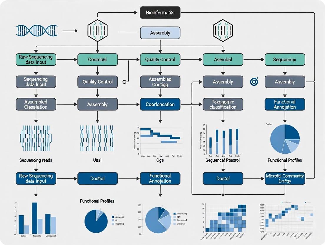
The computational workflow for shotgun metagenomics is complex and can be divided into several core modules. The graph below maps the logical flow and key decision points in a comprehensive bioinformatics pipeline.
Protocol Steps:
Quality Control and Preprocessing:
Host DNA Decontamination:
- Software: KneadData, Bowtie2 [4].
- Action: Align reads to the host reference genome (e.g., human, mouse) using Bowtie2. Discard all reads that align to the host to reduce contamination and focus computational resources on non-host sequences.
Taxonomic Profiling (Read-Based):
Functional Profiling (Read-Based):
Metagenome Assembly (Assembly-Based):
Binning and Metagenome-Assembled Genomes (MAGs):
- Software: MetaWRAP [4].
- Action: Group assembled contigs that likely originate from the same organism based on sequence composition (k-mers) and abundance across samples. This process, called binning, allows for the recovery of draft genomes from uncultured organisms.
The Scientist's Toolkit: Essential Research Reagents and Software
A successful shotgun metagenomics study relies on a suite of bioinformatics tools and reference databases. The following table catalogs key resources.
Table 2: Essential tools and databases for a shotgun metagenomics pipeline
| Category | Tool/Resource | Primary Function | Key Reference/Resource |
|---|---|---|---|
| Quality Control | FastQC | Quality assessment of raw sequencing reads | [7] [4] |
| fastp | Fast, all-in-one preprocessor for quality control and adapter trimming | [4] | |
| Host Removal | KneadData | Pipeline for removing host-associated sequences | [4] |
| Bowtie2 | Ultrafast, memory-efficient short read aligner for host read alignment | [4] | |
| Taxonomic Profiling | Kraken2 | Taxonomic classification of reads using k-mer matches | [4] [8] |
| Bracken | Bayesian estimation of species abundance from Kraken2 output | [4] | |
| MetaPhlAn4 | Profiling microbial composition using unique clade-specific markers | [4] | |
| Functional Profiling | HUMAnN3 | Profiling the abundance of microbial metabolic pathways | [4] [8] |
| Assembly & Binning | MEGAHIT | Metagenome assembler for large and complex datasets | [4] |
| MetaWRAP | A flexible pipeline for metagenome binning and refinement | [4] | |
| Gene Annotation | eggNOG-mapper | Functional annotation of genes using orthology | [4] [8] |
| Reference Databases | Greengenes2, SILVA | Curated databases of ribosomal RNA genes | [6] |
| RefSeq/GTDB | Comprehensive genome databases for taxonomic classification | ||
| UniRef90, MetaCyc | Protein family and metabolic pathway databases |
Integrated pipelines like EasyMetagenome [4] and the Sydney Informatics Hub workflow [7] bundle many of these tools into cohesive, scalable workflows, significantly reducing the burden of software deployment and ensuring reproducibility.
Shotgun metagenomics and amplicon sequencing are complementary yet distinct tools for microbial community analysis. Amplicon sequencing remains a powerful, cost-effective method for large-scale taxonomic surveys, particularly when focusing on well-characterized phylogenetic markers. However, shotgun metagenomics offers a transformative advantage by providing a comprehensive view of the microbiome, enabling high-resolution taxonomic assignment, functional potential analysis, and the reconstruction of metagenome-assembled genomes without prior cultivation [3] [4].
The choice of method should be guided by the research question. For projects requiring deep functional insights, strain-level discrimination, or the discovery of novel genes and pathways, shotgun metagenomics is the unequivocal choice. As sequencing costs continue to decline and bioinformatics pipelines become more standardized and accessible, shotgun metagenomics is poised to become the gold standard for in-depth microbiome investigation in drug development, clinical diagnostics, and beyond.
Shotgun metagenomics has revolutionized the study of microbial communities, enabling researchers to investigate microorganisms directly from their natural environments without the need for cultivation [9]. The analysis of these complex datasets relies on core computational approaches, each with distinct strengths and applications. This application note provides a detailed comparative analysis of the three principal analytical frameworks: read-based, assembly-based, and detection-based approaches. We frame this comparison within the context of developing robust bioinformatics pipelines for metagenomic research, offering structured experimental protocols, performance metrics, and implementation guidelines tailored for researchers, scientists, and drug development professionals. The choice of analytical strategy significantly impacts downstream interpretations, making selection criteria a critical consideration for study design [10].
Comparative Analysis of Approaches
Conceptual Foundations and Applications
Read-based approaches analyze unassembled sequencing reads, comparing them directly against reference databases for taxonomic classification and functional profiling [10]. This method is particularly valuable for quantitative community profiling when relevant references are available [9]. Tools such as Kraken2, Centrifuge, and MetaPhlAn2 operate within this paradigm, identifying organisms through alignment to clade-specific marker genes or k-mer matches [9] [11].
Assembly-based approaches attempt to reconstruct longer genomic segments (contigs) from short reads before analysis [10]. This workflow typically involves quality control, co-assembly of multiple samples, binning contigs into genomes, and subsequent gene annotation [12]. Popular assemblers include MEGAHIT, MetaSPAdes, and IDBA-UD, which are specifically designed for metagenomic data [9] [13]. This approach enables researchers to recover novel genomes and study genetic elements in their genomic context.
Detection-based approaches prioritize high-precision identification of specific organisms, often pathogens, with lower sensitivity compared to other methods [10]. These workflows typically employ alignment or k-mer based matching against curated datasets followed by heuristic classification methods [10]. This approach is particularly valuable in clinical diagnostics where confirming the presence of specific pathogens is critical.
Table 1: Core Characteristics of Metagenomic Analytical Approaches
| Feature | Read-based | Assembly-based | Detection-based |
|---|---|---|---|
| Primary Application | Bulk taxonomic/functional composition | Genomic context, novel genome recovery | High-confidence pathogen detection |
| Typical Questions | How do communities differ between sites/treatments? | What are metabolic capabilities of specific microbes? | Are known pathogens present in the sample? |
| Key Advantages | Fast, memory-efficient, quantitative | Recovers novel sequences, enables genomic analysis | High specificity, low false positive rate |
| Limitations | Limited by reference databases | Computationally intensive, challenging for complex communities | Limited to known targets, lower sensitivity |
| Representative Tools | Kraken2, Centrifuge, MetaPhlAn2 | MEGAHIT, MetaSPAdes, MaxBin | Taxonomer, Surpi, One Codex |
Performance Metrics and Benchmarking
Comparative studies demonstrate that the performance of these approaches varies significantly depending on the dataset characteristics and analytical goals. In a comprehensive benchmark of classification tools for long-read datasets, general-purpose mappers like Minimap2 achieved similar or better accuracy than best-performing specialized classification tools, though they were significantly slower than kmer-based methods [11]. The random forest technique has shown promising results as a suitable classifier, with models developed from read-based taxonomic profiling achieving 91% accuracy with a 95% confidence interval between 80% and 93% [9].
Assembly-based approaches face unique challenges in metagenomic contexts compared to single-genome assembly. The unknown abundance and diversity in samples complicate graph simplification, as low-coverage nodes may originate from genuine low-abundance genomes rather than sequencing errors [13]. Metagenomic abundance often follows a power law distribution, meaning many species occur with similarly low abundances, making distinguishing them problematic [13].
Detection-based approaches, particularly when combined with enrichment techniques, can significantly improve sensitivity. Capture panels can increase sensitivity by at least 10-100-fold over untargeted sequencing, making them suitable for detecting low viral loads (60 genome copies per ml) [14]. However, this enhanced sensitivity for targeted organisms comes at the cost of missing novel or unexpected pathogens not included in the panel.
Table 2: Performance Comparison Across Metagenomic Approaches
| Metric | Read-based | Assembly-based | Detection-based |
|---|---|---|---|
| Sensitivity | Limited for novel organisms | High for abundant community members | Excellent for targeted organisms |
| Specificity | Database-dependent | High with quality binning | Very high |
| Computational Demand | Low to moderate | Very high | Low to moderate |
| Reference Dependency | High | Low | Very high |
| Novel Discovery Potential | Limited | High | Very limited |
Detailed Experimental Protocols
Read-based Analysis Protocol
Sample Preparation and Sequencing
- Extract DNA/RNA using kits that preserve integrity of microbial nucleic acids
- Perform library preparation with unique dual indices to enable sample multiplexing
- Sequence using Illumina short-read or Nanopore long-read platforms
- Include appropriate controls (negative, positive, internal standards)
Quality Control and Preprocessing
- Demultiplex samples using barcode information (e.g.,
iu-demultiplexwith barcode file) [12] - Perform quality filtering with tools like
iu-filter-quality-minochefor large-insert libraries [12] - Remove adapter sequences and trim low-quality bases
- For host-associated samples, consider host DNA depletion methods
Taxonomic Profiling
- Select appropriate reference database (RefSeq, GTDB, custom)
- Run taxonomic classifier (Kraken2, Centrifuge, or MetaPhlAn2)
- For k-mer based tools, use Bracken for abundance estimation [11]
- For long reads, consider Minimap2 or Ram for alignment-based classification [11]
Downstream Analysis
- Import abundance tables into R/Python for statistical analysis
- Perform differential abundance testing between sample groups
- Conduct multivariate analysis (PCoA, PERMANOVA) for community comparisons
- Visualize results using heatmaps, bar plots, and ordination diagrams
Assembly-based Analysis Protocol
Data Preparation a. Perform quality control as in read-based protocol b. For multiple samples, consider co-assembly to maximize recovery c. Normalize read coverage to reduce computational complexity
Metagenomic Assembly
- Select assembler based on data type and resources:
- Execute assembly with optimized parameters:
- Assess assembly quality with N50, contig counts, and completeness metrics
Binning and Genome Resolution
- Map reads back to contigs for abundance estimation (Bowtie2, BBmap) [10]
- Perform metagenomic binning using multiple algorithms:
- MetaBAT2 for abundance-aware binning
- MaxBin2 for universal single-copy gene-based binning
- CONCOCT for sequence composition and coverage integration
- Consolidate bins using DAS Tool to generate non-redundant set
- Assess bin quality with CheckM for completeness and contamination
Gene Prediction and Annotation
- Identify open reading frames with Prodigal or MetaGeneMark [10]
- Annotate against functional databases (KEGG, COG, Pfam)
- Conduct pathway analysis and metabolic reconstruction
- Compare genomes across samples using average nucleotide identity
Reference-Guided Assembly Protocol
Reference Selection
- Identify relevant references from NCBI, GTDB, or specialty collections
- Use marker genes (e.g., single-copy core genes) to identify candidate genomes [15]
- Filter references based on sample-specific relevance
- Cluster references to reduce redundancy (e.g., with MinHash) [15]
Read Mapping and Assembly
- Align reads to reference genomes using BWA-MEM or Minimap2
- Identify coverage breaks and structural variations
- Generate sample-specific contigs using polishing algorithms
- "Mix and match" segments from multiple references for pangenome representation [15]
Validation and Quality Assessment
- Compare with de novo assemblies for completeness
- Validate with orthogonal methods (qPCR, culture)
- Assess contiguity metrics (NG50, NGA50) [15]
Workflow Visualization
Figure 1: Comparative Workflows for Metagenomic Analysis Approaches. Each approach begins with raw sequencing reads but follows distinct analytical pathways with different tool requirements and output types.
The Scientist's Toolkit
Table 3: Essential Research Reagents and Computational Tools
| Category | Item | Specification/Version | Application Notes |
|---|---|---|---|
| Wet Lab Reagents | NEBNext Microbiome DNA Enrichment Kit | E2612L | Depletes methylated host DNA, improves microbial detection [14] |
| KAPA RNA HyperPrep with RiboErase | KK8561 | rRNA depletion for RNA metagenomics, preserves host transcriptome [14] | |
| Twist Comprehensive Viral Research Panel | N/A | Targets 3153 viruses, increases sensitivity 10-100x [14] | |
| xGen UDI-UMI Adapters | 10005903 | Unique dual indices for sample multiplexing, reduces index hopping [14] | |
| Computational Tools | MEGAHIT | v1.0.6+ | Efficient metagenomic assembler, suitable for large datasets [12] |
| Kraken2/Bracken | v2.0+ | Fast kmer-based classification with abundance estimation [11] | |
| Minimap2 | v2.0+ | Versatile aligner for long reads, effective for metagenomics [11] | |
| MetaBAT2 | v2.0+ | Metagenomic binning tool using abundance and composition [10] | |
| CheckM | v1.0+ | Assesses completeness/contamination of genome bins [10] | |
| Reference Databases | GTDB | Release 200+ | Genome Taxonomy Database, standardized bacterial/archaeal taxonomy |
| RefSeq | Updated regularly | NCBI Reference Sequence Database, comprehensive genome collection | |
| UniProt | Updated regularly | Protein sequence and functional information [10] | |
| Quality Control | FastQC | v0.11+ | Quality control visualization for sequencing data |
| MultiQC | v1.0+ | Aggregates results from multiple tools into single report |
Implementation Considerations
Computational Resource Requirements
The computational demands of these approaches vary significantly. Kmer-based tools generally offer the fastest processing times with moderate memory requirements, while general-purpose mappers like Minimap2 provide slightly better accuracy but at significantly slower speeds [11]. Assembly-based approaches are the most computationally intensive, with memory requirements often scaling with dataset size and complexity [13]. For large-scale projects, assembly may require high-memory nodes (≥512GB RAM) and days of processing time, whereas read-based classification can often be completed in hours on standard servers.
Selection Guidelines
The choice of analytical approach should be guided by research questions and sample characteristics:
- Clinical diagnostics with known pathogen suspects: Detection-based approaches offer the highest specificity and rapid turnaround [10] [14]
- Community ecology studies: Read-based approaches efficiently characterize taxonomic and functional differences between sample groups [9]
- Novel genome discovery: Assembly-based approaches enable recovery of previously uncharacterized microorganisms [13] [15]
- Low biomass samples: Targeted enrichment combined with detection-based methods provides necessary sensitivity [14]
- Mixed communities with related strains: Reference-guided assembly approaches can leverage existing genomes to improve reconstructions [15]
For comprehensive studies, hybrid approaches often yield the best results, using multiple methods to compensate for individual limitations. A common strategy employs read-based analysis for initial community assessment followed by assembly-based methods for in-depth characterization of key community members.
The three core analytical approaches for metagenomics—read-based, assembly-based, and detection-based—each offer distinct advantages for different research scenarios. Read-based methods provide efficient community profiling, assembly-based approaches enable novel genome discovery, and detection-based methods deliver high-specificity pathogen identification. The optimal choice depends on research objectives, sample characteristics, and computational resources. As metagenomic applications expand in research and clinical settings, understanding these fundamental approaches and their appropriate implementation becomes increasingly critical for generating robust, reproducible microbiological insights. Future methodology developments will likely focus on hybrid approaches that combine the strengths of each method while addressing challenges of scalability, accuracy, and interpretation.
Typical Workflows and Research Questions Addressed by Each Method
Metagenomics, a term first coined by Handelsman in 1998, refers to "the genomes of the total microbiota found in nature" and involves obtaining sequence data directly from environmental samples [16]. This culture-independent approach has become a cornerstone of modern microbiology, enabling researchers to explore microbial communities in diverse habitats, from the human gut to soil and aquatic environments [17]. The field primarily utilizes two fundamental sequencing strategies: targeted (amplicon) sequencing and shotgun metagenomic sequencing. Each method offers distinct advantages and addresses specific research questions, with the choice between them depending on factors such as research objectives, resolution requirements, and budgetary constraints [18].
Targeted metagenomics, often called metagenetics, focuses on sequencing taxonomically informative genetic markers, typically the 16S rRNA gene for prokaryotes or the ITS region for fungi [19]. This approach provides a cost-effective means for characterizing microbial community composition and diversity. In contrast, shotgun metagenomics involves randomly sequencing all DNA fragments from a sample, enabling comprehensive analysis of both taxonomic content and functional potential [18]. The following sections provide a detailed examination of these methodologies, their workflows, applications, and the bioinformatics pipelines required to interpret the resulting data.
Targeted (Amplicon) Metagenomics
Research Questions and Applications
Targeted metagenomics, predominantly using 16S rRNA gene sequencing, is the preferred method for studies focusing primarily on microbial community composition and diversity. The 16S rRNA gene contains conserved regions that facilitate primer binding and hypervariable regions that provide taxonomic discrimination, making it an ideal biomarker for prokaryotic identification [17]. This approach addresses specific research questions including:
Microbial Community Profiling: Determining the taxonomic composition and relative abundance of microorganisms in a given environment. For example, studies have successfully used 16S sequencing to characterize rhizosphere microbial communities of crops like rice, wheat, and legumes [17], as well as to identify bacterial wilt disease pathogens in plants [17].
Comparative Diversity Analysis: Investigating how microbial communities differ across various conditions, time points, or habitats. This includes studies examining the effects of dietary interventions on gut microbiota or environmental perturbations on soil microbiomes.
Pathogen Identification and Diagnostics: Detecting and identifying pathogenic organisms in clinical, agricultural, or environmental samples. The high sensitivity of targeted sequencing makes it valuable for outbreak tracing and disease diagnostics [17].
The principal advantage of targeted metagenomics lies in its cost-effectiveness and lower sequencing depth requirements, enabling higher sample throughput for diversity studies. However, its limitations include primer bias affecting amplification efficiency and restricted taxonomic resolution, which often fails to reliably distinguish beyond the genus level for many taxa [20].
Experimental Protocol
The experimental workflow for targeted metagenomics follows a structured pathway from sample collection to sequencing:
- Sample Collection: The process begins with careful selection and collection of the target sample (e.g., soil, water, clinical specimens). Sample integrity is maintained through immediate processing or proper preservation to prevent microbial community shifts [17].
- DNA Isolation: Community DNA is extracted using methods appropriate for the sample type. This critical step often incorporates enzymatic (e.g., lysozyme, lysostaphin, mutanolysin) and mechanical lysis to address the diverse cell wall structures present in mixed microbial communities [17].
- PCR Amplification: Using consensus primers targeting conserved regions of the 16S rRNA gene (e.g., V3-V4 or V4-V5 hypervariable regions), the taxonomic marker is amplified. Appropriate controls are essential to detect potential contamination [17].
- Library Preparation and Sequencing: Amplified products are prepared for sequencing by adding platform-specific adapters. The library is quantified using methods such as qPCR or Bioanalyzer systems before undergoing high-throughput sequencing on platforms such as Illumina MiSeq or Ion Torrent [17].
Bioinformatics Pipelines and Analysis
The analysis of targeted metagenomics data involves multiple processing steps, which can be broadly categorized into "clustering-first" and "assignment-first" approaches [19]. The following workflow diagram illustrates the key stages and tools involved in this process:
Figure 1: Bioinformatics Workflow for Targeted Metagenomics
As illustrated in Figure 1, the analytical process begins with quality control and preprocessing of raw sequencing reads to remove artifacts and errors. The subsequent analysis branches into two methodological approaches:
Clustering-First Approaches: Tools such as DADA2, QIIME 2, and Mothur employ an initial step where sequences are clustered into Operational Taxonomic Units (OTUs) or denoised into Amplicon Sequence Variants (ASVs) based on sequence similarity. Representative sequences from each cluster are then taxonomically classified by comparison against reference databases [20] [19].
Assignment-First Approaches: Emerging tools like Kraken 2 and PathoScope 2 use an alternative method where reads are first classified against a reference database using k-mer matching or read mapping, before being grouped into taxonomic units [20] [19].
Recent benchmarking studies using mock microbial communities have demonstrated that assignment-first tools like Kraken 2 and PathoScope 2 can outperform traditional clustering-first approaches in species-level taxonomic assignments, especially when paired with comprehensive reference databases such as SILVA or RefSeq [20].
Table 1: Comparison of Bioinformatics Pipelines for Targeted Metagenomics
| Pipeline | Approach | Reference Databases | Strengths | Species-Level Accuracy |
|---|---|---|---|---|
| QIIME 2 | Clustering-first | Greengenes, SILVA, RDP | User-friendly interface, extensive plugins | Moderate [20] |
| DADA2 | Clustering-first | SILVA, RDP, Greengenes | High-resolution ASVs, precise error correction | Moderate [20] |
| Mothur | Clustering-first | SILVA, RDP, Greengenes | Comprehensive workflow, SOP guidance | Moderate [20] |
| Kraken 2 | Assignment-first | Kraken 2 Standard, SILVA | Fast k-mer based classification, sensitive | High [20] |
| PathoScope 2 | Assignment-first | RefSeq | Bayesian read reassignment, handles ambiguities | High [20] |
Shotgun Metagenomics
Research Questions and Applications
Shotgun metagenomic sequencing provides a comprehensive view of all genes and organisms in a complex sample, enabling researchers to address broader research questions that extend beyond taxonomic classification to functional potential [18]. This approach is particularly valuable for:
Functional Gene Annotation: Identifying and characterizing metabolic pathways, virulence factors, antimicrobial resistance genes, and other functional elements within microbial communities. For example, shotgun sequencing has been applied to surveil biological impurities and antimicrobial resistance genes in vitamin-containing food products [21].
Unculturable Microorganism Discovery: Studying microorganisms that cannot be cultivated in laboratory settings, potentially revealing novel taxa and genes. This has led to the discovery of novel antimicrobials like Terbomycine A and B, and bacterial enzymes such as NHLase [17].
Metagenome-Assembled Genomes (MAGs): Reconstructing genomes from complex microbial communities without the need for isolation and cultivation. Recent advances in long-read sequencing and bioinformatics have enabled recovery of more high-quality, single-contig MAGs [22].
Strain-Level Differentiation: Discriminating between closely related microbial strains, which is crucial for outbreak investigations and understanding microbe-disease relationships.
The key advantage of shotgun metagenomics is its ability to simultaneously assess both taxonomic composition and functional capabilities of microbial communities. However, this comprehensive approach requires deeper sequencing, resulting in higher costs and more complex computational requirements compared to targeted methods [18].
Experimental Protocol
The shotgun metagenomics workflow involves the following key experimental steps:
Sample Collection and DNA Extraction: Similar to targeted approaches, samples are collected with consideration for temporal and geographical factors. DNA extraction must be comprehensive to capture genetic material from diverse microorganisms, often requiring rigorous lysis protocols [17].
Library Preparation without Target Enrichment: Unlike targeted metagenomics, shotgun sequencing does not involve PCR amplification of specific markers. Instead, total DNA is fragmented physically or enzymatically, and sequencing adapters are ligated to the fragments. Protocols vary by platform, such as the NEBNext Ultra II DNA library prep kit for Illumina [23] or the Ligation Sequencing Kit for Oxford Nanopore platforms [24].
High-Throughput Sequencing: Libraries are sequenced using platforms such as Illumina NovaSeq, PacBio Sequel II, or Oxford Nanopore GridION/MinION. Sequencing depth is critical, with recommendations ranging from millions to billions of reads depending on complexity and objectives [23] [18].
Specialized Protocols: Advanced applications may require specialized approaches. For example, the FDA protocol for bacterial enrichments using Oxford Nanopore R10 flow cells enables multiplexing of up to 16 samples per flow cell [24]. HiFi shotgun metagenomics with PacBio systems provides long-read data that improves genome completeness and enables recovery of more species and MAGs [22].
Bioinformatics Pipelines and Analysis
The analysis of shotgun metagenomic data involves a more complex workflow than targeted approaches, with multiple specialized steps as illustrated below:
Figure 2: Bioinformatics Workflow for Shotgun Metagenomics
As shown in Figure 2, shotgun metagenomics analysis involves several interconnected pathways:
Read Preprocessing and Host Removal: Quality control tools like FastQC and fastp remove adapters and low-quality reads. Host DNA contamination is eliminated using tools like Kraken2 with custom host databases or minimap2 [23] [25].
Taxonomic Profiling: Processed reads are directly classified using tools such as the DRAGEN Metagenomics Pipeline or Kraken 2, which perform taxonomic classification and provide abundance estimates [18] [25].
Assembly and Binning: For functional analysis, quality-filtered reads are assembled into contigs using tools like MEGAHIT or metaSPAdes. Contigs are then binned into metagenome-assembled genomes (MAGs) using tools such as MAXBIN [25].
Gene Prediction and Functional Annotation: Open reading frames are predicted from assembled contigs using tools like Prodigal or MetaGeneMark. Predicted genes are functionally annotated by comparison against databases including KEGG, eggNOG, and CAZy using alignment tools like DIAMOND or BLAST+ [25].
Recent advances in shotgun metagenomics analysis have demonstrated significant improvements in outcomes. Updated bioinformatics pipelines for HiFi shotgun metagenomics data have shown 162-808% increases in species detection and 18-48% improvements in high-quality MAG recovery compared to previous methods [22].
Table 2: Comparison of Bioinformatics Pipelines for Shotgun Metagenomics
| Pipeline/Tool | Application | Key Features | Reference Databases | Performance |
|---|---|---|---|---|
| DRAGEN Metagenomics | Taxonomic profiling | Optimized for Illumina data, efficient processing | Custom curated databases | High accuracy for species identification [18] |
| Kraken 2 | Taxonomic profiling | Ultra-fast k-mer classification, sensitive | Kraken 2 Standard, customizable | High species-level accuracy [20] |
| PathoScope 2 | Taxonomic profiling | Bayesian reassignment of ambiguous reads | RefSeq | Accurate strain-level identification [20] |
| MGS-Fast | Functional annotation | Rapid alignment to microbial gene catalogs | Custom gene catalogs | Identifies differential functional genes [25] |
| Prodigal | Gene prediction | Prokaryotic gene prediction, precise start/stop codon identification | None (ab initio predictor) | Accurate ORF detection [25] |
Research Reagent Solutions
The following table outlines essential reagents and materials used in shotgun metagenomics library preparation and sequencing, based on the Oxford Nanopore Platform protocol [24]:
Table 3: Essential Research Reagents for Shotgun Metagenomics
| Component | Function | Example Product |
|---|---|---|
| Native Barcode | Sample multiplexing and identification | Native Barcode Plate (NB01-96) |
| DNA Control Sample | Sequencing process control | DNA Control Sample (DCS) |
| Native Adapter | Library attachment to sequencing matrix | Native Adapter (NA) |
| Sequencing Buffer | Provides optimal chemical environment | Sequencing Buffer (SB) |
| Library Beads | Purification and size selection of DNA fragments | AMPure XP Beads |
| Elution Buffer | Final resuspension of purified library | Elution Buffer (EB) |
| End Repair Mix | Prepares DNA fragments for adapter ligation | NEBNext UltraII End repair/dA-tailing Module |
| Ligation Master Mix | Catalyzes adapter ligation to DNA fragments | NEB Blunt/TA Ligase Master Mix |
| Flow Cell | Platform-specific sequencing matrix | Oxford Nanopore R10 Flow Cell |
Targeted and shotgun metagenomics represent complementary approaches with distinct strengths and applications in microbial community analysis. Targeted metagenomics, primarily using 16S rRNA gene sequencing, provides a cost-effective method for comprehensive taxonomic profiling and diversity analysis across large sample sets. In contrast, shotgun metagenomics offers unparalleled insights into both taxonomic composition and functional potential, enabling discovery of novel genes, pathways, and metagenome-assembled genomes.
The choice between these methods should be guided by specific research questions, resources, and analytical requirements. Targeted approaches remain ideal for studies focused primarily on community composition and dynamics, while shotgun methods are essential for investigating functional capabilities and genetic potential. As sequencing technologies continue to advance and bioinformatics pipelines become more sophisticated, both methods will continue to evolve, providing increasingly powerful tools for exploring the microbial world across diverse research contexts from human health to environmental monitoring.
Shotgun metagenomic sequencing represents a powerful, culture-independent method for analyzing the totality of genomic material within a microbial sample, enabling comprehensive insights into both taxonomic composition and functional potential [26]. Unlike targeted 16S rRNA gene sequencing, which focuses on specific hypervariable regions, shotgun sequencing randomly fragments all DNA, providing sequences that can be assembled into contigs and potentially complete genomes, while also allowing for superior species-level resolution [27]. The primary analytical outputs of this approach are taxonomic profiles, which detail the identity and relative abundance of microorganisms present, and Metagenome-Assembled Genomes (MAGs), which are reconstructed genomes of individual microbial population members derived from the assembly of sequencing reads [26]. These outputs are foundational for exploring the structure and function of microbial communities in diverse environments, from the human gut to complex ecosystems. The reliability of these outputs, however, is intrinsically linked to the bioinformatics pipelines and computational tools used for processing, each employing distinct methodologies—such as k-mer-based classification, marker gene analysis, and assembly-based approaches—that can significantly impact the final results [27] [28]. This document outlines the key outputs, benchmarks performance across available tools, and provides detailed protocols for generating robust taxonomic profiles and MAGs.
Benchmarking Pipelines and Performance Metrics
Choosing an appropriate bioinformatics pipeline is critical, as the performance of taxonomic classifiers and profilers varies significantly in terms of sensitivity, precision, and accuracy of abundance estimation. Benchmarking studies using mock microbial communities with known compositions provide essential objective assessments of these tools.
Table 1: Performance of Shotgun Metagenomics Taxonomic Classification Pipelines
| Pipeline Name | Classification Approach | Key Features | Reported Performance Highlights |
|---|---|---|---|
| bioBakery (MetaPhlAn4) | Marker gene & MAG-based [27] | Utilizes clade-specific marker genes and species-level genome bins (SGBs) [27]. Integrated within a comprehensive suite of tools [28]. | Ranked best overall in a recent assessment using multiple mock communities, demonstrating high accuracy across most metrics [27]. |
| JAMS | Assembly-assisted, k-mer-based (Kraken2) [27] | Performs whole-genome assembly and uses Kraken2 for classification. Provides detailed genomic analysis [27]. | Achieved among the highest sensitivity for detecting species, though may require validation against false positives [27]. |
| WGSA2 | k-mer-based (Kraken2) [27] | Offers optional genome assembly. Focuses on taxonomic profiling from reads [27]. | Showed high sensitivity in benchmarking studies, comparable to JAMS [27]. |
| Woltka | Operational Genomic Unit (OGU) [27] | Classifies based on phylogeny and evolutionary lineage of reference genomes. Does not perform assembly [27]. | A newer classifier that offers a phylogenetically-aware alternative to k-mer and marker-based methods [27]. |
| BugSeq | Long-read optimized [29] | Designed specifically for long-read (PacBio HiFi, ONT) data. | Demonstrated high precision and recall with PacBio HiFi data, detecting all species down to 0.1% abundance without filtering [29]. |
| MEGAN-LR & DIAMOND | Long-read optimized [29] | Uses alignment-based classification for long-read datasets. | Along with BugSeq and sourmash, displayed high precision and recall on long-read datasets without requiring heavy filtering [29]. |
Table 2: Comparative Analysis of Classification Methodologies
| Methodology | Representative Tools | Advantages | Disadvantages |
|---|---|---|---|
| Marker Gene-Based | MetaPhlAn4 [27] [28] | Computationally efficient, low false positive rate, provides direct relative abundance estimates [27]. | Limited to organisms with known marker genes; may miss novel taxa [27]. |
| k-mer-Based | Kraken2, WGSA2, JAMS [27] [28] | High sensitivity, uses comprehensive reference databases, can classify a broad range of reads [27]. | Can produce false positives; often requires filtering; computationally intensive for large databases [29]. |
| Alignment-Based (for Long Reads) | MEGAN-LR, MetaMaps [29] | Leverages long-range information in reads (multiple genes), high accuracy for high-quality long reads [29]. | Performance can be affected by read quality and length; computationally demanding [29]. |
| Assembly-Based | MEGAHIT, metaSPAdes | Enables reconstruction of genomes (MAGs) and discovery of novel genes [26]. | Computationally very intensive; assembly of complex communities can be fragmented and challenging [26]. |
Workflow Diagram: From Raw Data to Key Outputs
The following diagram illustrates the standard bioinformatics workflow for processing shotgun metagenomics data, from raw sequencing reads to the key outputs of taxonomic profiles and MAGs, integrating the tools and pipelines discussed.
Diagram Title: Shotgun Metagenomics Analysis Workflow
Detailed Experimental Protocols
Protocol 1: Generating a Taxonomic Profile with bioBakery
The bioBakery suite, specifically the MetaPhlAn4 tool, is a widely used and well-performing pipeline for taxonomic profiling from shotgun metagenomic reads [27] [28]. This protocol is adapted from established workflows and benchmarking studies.
Principle: MetaPhlAn4 uses a database of clade-specific marker genes to taxonomically assign sequencing reads, providing species-level resolution and relative abundance estimates. It incorporates both known and unknown species-level genome bins (SGBs) for improved coverage of microbial diversity [27].
Materials:
- Computing Environment: A computer with a command-line interface (Linux or macOS) or access to a high-performance computing (HPC) cluster. Basic command-line knowledge is required [30].
- Container Software: Docker or Singularity installed to ensure reproducibility [28].
- Input Data: Quality-controlled and host-depleted paired-end or single-end sequencing reads in FASTQ format.
- Database: The MetaPhlAn4 database, which can be downloaded automatically on first run or manually.
Procedure:
- Quality Control and Host Depletion: Begin with raw FASTQ files. Use Trimmomatic to remove adapter sequences and low-quality bases. If the sample is host-derived (e.g., from a human biopsy), use a tool like HISAT2 to align reads against the host genome (e.g., human GRCh38) and retain only the unmapped reads for downstream analysis [28].
- Run MetaPhlAn4: Execute the following basic command, replacing the placeholders with your file paths.
- For paired-end reads: Use
--nprocto specify the number of parallel processing threads for faster execution. - The
--bowtie2outflag saves the intermediate Bowtie2 alignment file for potential re-use.
- For paired-end reads: Use
- Interpret Output: The primary output
taxonomic_profile.txtis a tab-separated file listing detected taxa from kingdom to species level, their unique taxonomic IDs, and their relative abundance in the sample.
Troubleshooting and Optimization:
- If many reads remain unclassified, consider that your sample may contain microbial lineages not well-represented in the standard MetaPhlAn4 database.
- For large-scale studies, consider using integrated pipelines like MeTAline, which wraps MetaPhlAn4 (and other tools like Kraken2) within a Snakemake workflow, automating the steps from quality control to profiling and ensuring reproducibility [28].
Protocol 2: Reconstructing Metagenome-Assembled Genomes (MAGs)
This protocol outlines the assembly-based pathway for reconstructing near-complete genomes from complex metagenomic samples, which allows for in-depth functional analysis and discovery of novel microorganisms [26].
Principle: Short sequencing reads are assembled into longer contiguous sequences (contigs). These contigs are then grouped ("binned") based on sequence composition (e.g., k-mer frequency, GC content) and abundance patterns across multiple samples, ultimately resulting in draft genomes for individual populations.
Materials:
- Input Data: High-quality, pre-processed sequencing reads (as from Protocol 1, Step 1). Deeper sequencing coverage is generally required for successful MAG recovery than for taxonomic profiling.
- Software:
- Assembler: MEGAHIT or metaSPAdes.
- Binner: MetaBAT2, MaxBin2, or CONCOCT.
- CheckM or similar for assessing MAG quality and completeness.
Procedure:
- De Novo Assembly: Assemble the quality-controlled reads into contigs. Example using MEGAHIT:
The final contigs are typically found in
assembly_output/final.contigs.fa. - Read Mapping: Map the original quality-controlled reads back to the assembled contigs to generate abundance information for each contig. This is typically done using Bowtie2 to create a BAM file, which is then sorted and indexed.
- Binning: Execute one or more binning tools on the contigs and the sorted BAM file to group contigs into putative genomes.
- Quality Assessment and Refinement: Evaluate the quality of the reconstructed MAGs using CheckM. CheckM will report estimates of completeness and contamination. High-quality MAGs are typically defined as those with >90% completeness and <5% contamination. Use these metrics to select the best-quality MAGs for downstream analysis.
Troubleshooting and Optimization:
- A high rate of fragmented assemblies can result from low sequencing depth or highly complex communities. Consider increasing sequencing depth or using a combination of assembly algorithms.
- Binners often perform better on different datasets; using a consensus approach (dereplicating results from multiple binners) can yield a more complete and higher-quality set of MAGs.
The Scientist's Toolkit: Essential Research Reagents and Materials
Table 3: Key Reagents, Databases, and Software for Shotgun Metagenomics
| Item Name | Type | Function and Application |
|---|---|---|
| Trimmomatic | Software Tool | Removes adapter sequences and low-quality bases from raw sequencing reads during the essential quality control step [28]. |
| Kraken2 Database | Reference Database | A comprehensive k-mer database used by classifiers like Kraken2, JAMS, and WGSA2 to assign taxonomy to reads or contigs [27] [28]. Can be customized to include specific genomes. |
| MetaPhlAn4 Database | Reference Database | A curated collection of clade-specific marker genes used by MetaPhlAn4 for highly efficient and specific taxonomic profiling and relative abundance estimation [27] [28]. |
| MetaBAT2 | Software Tool | A widely used tool for binning assembled contigs into Metagenome-Assembled Genomes (MAGs) based on sequence composition and abundance across samples [26]. |
| CheckM | Software Tool | Assesses the quality of reconstructed MAGs by estimating completeness and contamination using a set of conserved, single-copy marker genes, which is critical for downstream analysis [26]. |
| MeTAline Pipeline | Integrated Workflow | A containerized Snakemake pipeline that integrates multiple tools (e.g., Trimmomatic, Kraken2, MetaPhlAn4, HUMAnN) into a single, reproducible workflow from reads to taxonomy and function [28]. |
| HUMAnN3 | Software Tool | Performs functional profiling of microbial communities by determining the abundance of microbial pathways from metagenomic data, often stratifying results by contributing species [28]. |
Building Your Pipeline: A Step-by-Step Workflow from Sample to Insight
The reliability of any shotgun metagenomics study is fundamentally contingent on the quality and precision of its initial, wet-lab phase. The pre-analytical steps—encompassing sample collection, nucleic acid extraction, and library preparation—form the foundational pillar upon which all subsequent bioinformatics analysis is built [31]. Errors or inconsistencies introduced at these stages can propagate through the entire workflow, leading to biased taxonomic profiles, compromised functional annotations, and ultimately, misleading biological conclusions [32] [33]. This application note provides a detailed protocol for these critical pre-analytical procedures, framed within the context of a comprehensive bioinformatics pipeline for shotgun metagenomics research. It is designed to equip researchers and drug development professionals with the methodologies to ensure the generation of high-quality, reproducible sequencing data.
Sample Collection and Preservation
The goal of sample collection is to obtain a representative microbial biomass while minimizing the introduction of contaminants and preserving the integrity of the nucleic acids.
Key Considerations
- Sample Type: The strategy must be tailored to the sample matrix (e.g., whole blood, plasma, tissue, environmental swabs) [32] [31]. For instance, blood stream infection diagnostics must contend with high levels of human background DNA, which can drastically reduce the sequencing depth of microbial pathogens [32].
- Biomass and Volume: Sufficient microbial biomass is critical. For low-biomass samples, the use of ultraclean reagents and "blank" sequencing controls is essential to distinguish true microbial signals from contamination [33]. The recommended volume for blood culture diagnostics is 40–60 mL, though molecular tests often use only 1–10 mL, which can impact detection sensitivity [32].
- Preservation and Storage: Immediate freezing at -80°C or use of appropriate stabilization buffers is recommended to prevent microbial growth or degradation post-collection.
This protocol is adapted from a study developing a shotgun metagenomics protocol for blood stream infections.
Materials:
- Fresh whole blood (WB) from healthy volunteers, collected in EDTA tubes.
- Bacterial strains (e.g., Staphylococcus aureus, Escherichia coli, Streptococcus pneumoniae)
- 0.85% NaCl solution
- Blood agar plates
Method:
- Culture and Standardize Inoculum:
- Culture bacterial strains overnight on blood agar plates at 36.5°C.
- Suspend bacterial colonies in 0.85% NaCl to a turbidity of 0.5 McFarland (approximately 10^8 CFU/mL).
- Perform serial 10-fold dilutions in 0.85% NaCl. Plate 100 µL of each dilution in triplicate to confirm the CFU/mL.
Spiking into Whole Blood:
- Combine EDTA-blood from volunteers in a falcon tube.
- Spike the WB with the prepared bacterial suspensions within the same hour of the blood draw to achieve final concentrations typically between 10^3 to 10^5 CFU/mL.
Preparation of Plasma Samples (Optional):
- To obtain plasma, centrifuge 5 mL of spiked WB at 180 g or 100 g for 10 minutes at room temperature.
- Carefully collect 1 mL of the supernatant (plasma) for downstream DNA extraction.
DNA Extraction and Human DNA Depletion
Efficient extraction of microbial DNA and concomitant depletion of host DNA is arguably the most critical step for sensitivity, particularly in clinical samples where host DNA can constitute over 75% of the total sequenced reads [31].
Experimental Comparison of Extraction Efficiency
A study evaluating DNA extraction for shotgun metagenomics from blood reported significant differences in performance based on sample matrix and bacterial species [32]. The key quantitative findings are summarized in the table below.
Table 1: Comparison of DNA Extraction Efficiency from Whole Blood vs. Plasma [32]
| Sample Matrix | Bacterial Read Yield | Method Reproducibility | Performance by Gram Stain | Human DNA Depletion (ddPCR for RPP30 gene) |
|---|---|---|---|---|
| Whole Blood (WB) | Higher | Less consistent | More efficient for Gram-positive bacteria (S. aureus, S. pneumoniae) | Variable efficiency |
| Plasma | Lower | More consistent, better reproducibility | Negative effect on Gram-negative bacteria (E. coli) | More consistent and efficient |
Materials:
- Molzym Blood Pathogen Kit
- Automatic extraction system (e.g., Arrow, Diasorin)
- Qubit dsDNA HS Assay Kit
- Nanodrop spectrophotometer
- Agilent TapeStation with gDNA ScreenTape assay
Method:
- Extract DNA from Whole Blood:
- Use the Blood Pathogen Kit combined with the add-on 10 complement to extract DNA from 10 mL of spiked WB. This kit includes a step for selective lysis of human cells and degradation of human DNA.
Extract DNA from Plasma:
- For 1 mL of plasma obtained in Section 2.2, use the Blood Pathogen Kit without the add-on 10 complement, following the manufacturer's instructions for automatic extraction.
DNA Elution and Storage:
- Elute the extracted DNA in 100 µL of the kit's elution buffer.
- Store the DNA at -80°C until library preparation.
DNA Quality and Quantity Assessment:
- Quantify DNA using the Qubit dsDNA HS assay.
- Assess Purity using a Nanodrop spectrophotometer (A260/A280 and A260/A230 ratios).
- Evaluate Fragment Size using the gDNA ScreenTape assay on an Agilent TapeStation.
Library Preparation for Nanopore Sequencing
Library preparation converts the extracted DNA into a format compatible with the sequencing platform. The choice of technology impacts turnaround time and application suitability.
This protocol enables same-day diagnostics, offering a short turnaround time meaningful in a clinical context.
Materials:
- Oxford Nanopore Rapid PCR Barcoding Kit (SQK-RPB004)
- AMPure XP beads
- MinION device with FLO-MIN106 R9.4 flowcell
Method:
- Library Input: Use 1–5 ng of extracted DNA as input, depending on the yield from the extraction step.
PCR Amplification and Barcoding:
- Perform the library preparation according to the manufacturer's instructions for the Rapid PCR Barcoding Kit.
- Modification: Increase the number of PCR cycles from the standard 14 to 24 cycles to enhance yield from low-biomass samples.
Clean-up:
- Incubate the library with AMPure XP beads and Tris-HCl buffer for 10 and 5 minutes, respectively (increased from the standard protocol to improve recovery).
Sequencing:
- Load the DNA library onto a FLO-MIN106 R9.4 flowcell.
- Sequence on a MinION device for 24 hours.
The Researcher's Toolkit: Essential Materials
Table 2: Key Research Reagent Solutions for Pre-analytical Workflow
| Item | Function | Example Product/Catalog Number |
|---|---|---|
| Blood Pathogen Kit | Integrated DNA extraction and human DNA depletion from whole blood and plasma. | Molzym Blood Pathogen Kit |
| Rapid PCR Barcoding Kit | Fast preparation of sequencing libraries for Oxford Nanopore platforms, enabling same-day turnaround. | Oxford Nanopore SQK-RPB004 |
| AMPure XP Beads | Solid-phase reversible immobilization (SPRI) beads for post-reaction clean-up and size selection. | Beckman Coulter AMPure XP |
| Qubit dsDNA HS Assay | Highly sensitive, specific fluorescent quantification of double-stranded DNA, crucial for low-concentration samples. | Thermo Fisher Scientific Qubit dsDNA HS Assay |
| gDNA ScreenTape Assay | Automated electrophoretic analysis of genomic DNA size distribution and integrity. | Agilent Technologies gDNA ScreenTape |
Workflow Visualization
The following diagram illustrates the complete pre-analytical workflow, from sample collection to a sequence-ready library, integrating the protocols described in this document.
In shotgun metagenomics, quality control (QC) and trimming form the critical foundation upon which all subsequent analysis relies. Raw sequencing data invariable contains artifacts—low-quality bases, adapter sequences, and contaminating DNA—that can significantly compromise downstream results including assembly, binning, and taxonomic profiling [34]. Effective QC procedures identify and remove these artifacts, preventing erroneous conclusions and ensuring the accuracy of microbial community analysis [34]. This protocol outlines comprehensive QC strategies, tools, and metrics essential for robust metagenomic research, forming an integral component of standardized bioinformatics pipelines for microbiome investigation.
Key Quality Metrics and Their Interpretation
Understanding and monitoring key quality metrics is fundamental for evaluating sequencing data. The table below summarizes the core metrics used in metagenomic QC.
Table 1: Key Quality Control Metrics for Shotgun Metagenomics
| Metric | Description | Interpretation | Common Thresholds |
|---|---|---|---|
| Quality Score (Q Score) | Logarithmic measure of base-calling accuracy [35] | Q20 = 99% accuracy (1% error); Q30 = 99.9% accuracy (0.1% error) [35] | Minimum Q20 for reliable analysis [36] |
| Contiguity | Measure of assembly completeness and continuity | N50: Length of the shortest contig at 50% of total assembly length | Higher values indicate better assembly [37] |
| Completeness | Percentage of single-copy marker genes found in a Metagenome-Assembled Genome (MAG) [37] | Indicates how much of a genome has been recovered | ≥90% for high-quality MAGs [37] |
| Contamination | Percentage of marker genes duplicated in a MAG, suggesting multiple genomes binned together [37] | Lower values indicate purer genome bins | <5% for high-quality MAGs [37] |
| Chimerism | Detection of sequences originating from different genomic backgrounds [37] | Suggests incorrectly joined sequences or bins | Lower values preferred; specific thresholds vary by tool |
Essential Tools for Quality Control and Trimming
A robust QC pipeline utilizes specialized tools at different processing stages. The selection of tools depends on the sequencing technology and specific analysis goals.
Table 2: Essential Tools for Metagenomic Quality Control and Trimming
| Tool | Primary Function | Key Features | Application Context |
|---|---|---|---|
| FastQC | Quality assessment of raw sequencing data [4] [34] | Provides visual reports on per-base quality, GC content, adapter contamination [34] | Initial quality check; pre- and post-trimming [4] |
| fastp | Quality control, filtering, and adapter removal [4] | Performs integrated adapter trimming, quality filtering, and correction [4] | Rapid preprocessing of short-read data [4] |
| KneadData | Removal of host contamination [4] | Identifies and removes reads mapping to host reference genomes [4] | Essential for host-associated microbiome studies (e.g., human gut) |
| Trimmomatic | Read trimming and adapter removal [38] | Uses sliding window approach for quality-based trimming [38] | Reliable preprocessing within larger workflows [38] |
| QUAST | Assembly quality assessment [37] [4] | Evaluates contiguity statistics and assembly completeness [37] | Post-assembly evaluation of contigs and MAGs [37] |
| CheckM2 | MAG quality assessment [37] | Estimates completeness and contamination using machine learning [37] | Bin evaluation and refinement [37] |
| BUSCO | MAG quality assessment [37] | Assesses completeness and duplication based on universal single-copy orthologs [37] | Bin evaluation and comparison [37] |
| QC-Chain | Holistic QC with contamination screening [34] | Provides de novo contamination identification and fast processing [34] | Comprehensive QC for complex metagenomic datasets [34] |
Standardized Workflow for Quality Control and Trimming
The following workflow diagram illustrates the sequential stages of a comprehensive QC process for shotgun metagenomics, integrating the tools and metrics previously described.
Workflow Title: Comprehensive QC and Trimming Pipeline for Shotgun Metagenomics
Initial Quality Assessment
Objective: Evaluate the raw sequencing data quality before any processing.
- Procedure:
- Run FastQC on raw sequencing files (FASTQ format).
- Examine the HTML report for key metrics:
- Per base sequence quality: Identify positions with poor quality scores.
- Per sequence quality scores: Assess overall read quality.
- Sequence length distribution: Confirm expected read lengths.
- Overrepresented sequences: Detect adapter contamination or other contaminants.
- K-mer content: Identify possible sequencing biases.
- Interpretation: This initial assessment determines the specific trimming and filtering parameters needed. Poor quality at read ends typically requires more aggressive trimming, while adapter contamination necessitates adapter removal.
Adapter Trimming and Quality Filtering
Objective: Remove adapter sequences, low-quality bases, and discard poor-quality reads.
- Procedure using fastp:
- Execute fastp with recommended parameters:
--cut_front --cut_tail --cut_window_size 4 --cut_mean_quality 20--length_required 50to discard very short fragments- Specify adapter sequences with
--adapter_fastaif known
- For paired-end data, include
--detect_adapter_for_peto automatically identify common adapters - Enable correction for paired-end data with
--correctionfor overlapping reads
- Execute fastp with recommended parameters:
- Quality Thresholds:
Host DNA Decontamination
Objective: Identify and remove reads originating from host DNA, which is crucial for host-associated microbiome studies.
- Procedure using KneadData:
- Prepare a reference database of the host genome (e.g., human GRCh38).
- Align reads to the host reference using Bowtie2 with sensitive parameters.
- Extract unmapped reads, which represent the microbial fraction.
- For samples with high host contamination (>90%), consider additional probabilistic filtering with tools like BMTagger [38].
- Validation:
- Monitor the percentage of reads remaining after host removal.
- Expected retention rates vary by sample type: typically 60-90% for stool samples, but may be as low as 10-30% for tissue biopsies.
Post-Cleaning Quality Assessment
Objective: Verify the effectiveness of QC procedures and ensure data quality before downstream analysis.
- Procedure:
- Run FastQC on the cleaned sequencing files.
- Compare reports before and after processing to confirm:
- Improved per-base quality scores
- Elimination of adapter sequences
- Appropriate sequence length distribution after trimming
- Generate quality metrics for the final cleaned dataset:
- Total number of reads and total bases
- Average read length and N50
- Overall GC content distribution
Assembly and MAG Quality Assessment
Objective: Evaluate the quality of assembled contigs and Metagenome-Assembled Genomes (MAGs).
- Procedure using MAGFlow framework:
- Run QUAST to evaluate assembly contiguity metrics (N50, total length, number of contigs) [37].
- Execute CheckM2 to estimate completeness and contamination of MAGs [37].
- Perform BUSCO analysis to assess gene space completeness based on universal single-copy orthologs [37].
- Run GUNC to detect chimerism in genome bins [37].
- Quality Standards for MAGs:
- High-quality MAGs: ≥90% completeness, <5% contamination [37].
- Medium-quality MAGs: ≥50% completeness, <10% contamination.
The Scientist's Toolkit: Research Reagent Solutions
Table 3: Essential Research Reagents and Kits for Metagenomic Sequencing
| Reagent/Kit | Function | Application Notes |
|---|---|---|
| ZymoBIOMICS DNA Kit | DNA extraction from complex samples | Maintains representative representation of community structure; suitable for difficult-to-lyse microbes |
| Nextflex Rapid XP DNA Seq Kit | Library preparation for Illumina platforms | Incorporates unique dual indexes to enable sample multiplexing and reduce index hopping [36] |
| ZR Bashing Bead Lysis Tubes | Mechanical disruption of microbial cells | Essential for breaking tough cell walls of Gram-positive bacteria and fungi [36] |
| Qubit HS DNA Kit | Accurate quantification of DNA concentration | Fluorometric method superior to spectrophotometry for quantifying low-concentration metagenomic DNA [36] |
| LabChip GX Touch Nucleic Acid Analyzer | Fragment size distribution analysis | Quality control check after library preparation to verify insert size and absence of adapter dimers [36] |
Troubleshooting and Optimization Guidelines
Addressing Common QC Challenges
Low Read Quality:
- If persistent quality drops at read ends, increase trimming stringency or truncate reads to a fixed length.
- For overall poor quality, consider requesting resequencing if the percentage of bases above Q20 falls below 70%.
High Host Contamination:
- For samples with >90% host DNA, use probabilistic filtering tools like BMTagger in addition to standard alignment-based approaches [38].
- Optimize wet-lab protocols to enrich for microbial biomass through differential centrifugation or filtration.
Insufficient Sequencing Depth:
- For complex environmental samples, ensure adequate sequencing depth (typically 5-10 Gb per soil sample, 1-5 Gb per gut sample).
- Use rarefaction analysis to determine if diversity has been adequately captured.
Pipeline Integration and Best Practices
Modern metagenomic analysis increasingly utilizes integrated pipelines that incorporate QC steps:
- EasyMetagenome: Provides a comprehensive workflow including quality control, host removal, and multiple analysis paths [4].
- MAGFlow: Specifically designed for quality assessment of MAGs through multiple validation tools [37].
- Reproducibility: Always document QC parameters and software versions. Use containerization (Docker/Singularity) and workflow managers (Nextflow/Snakemake) to ensure reproducible results [37].
Rigorous quality control and trimming are not merely preliminary steps but fundamental components that determine the success of any shotgun metagenomics study. By implementing the protocols outlined in this document—from initial quality assessment through host decontamination to final assembly validation—researchers can ensure the reliability of their taxonomic and functional analyses. The integration of these QC processes into standardized, reproducible bioinformatics pipelines empowers robust microbiome research across diverse fields from clinical diagnostics to environmental monitoring.
Host DNA Removal and Contaminant Filtration Strategies
In shotgun metagenomics, the detection and accurate characterization of microbial communities is often confounded by the presence of host DNA and other contaminants. This challenge is particularly acute in low-biomass samples, such as those from the respiratory tract, where host DNA can constitute over 99.9% of sequenced material, thereby obscuring microbial signals and compromising analytical sensitivity [39]. The development of robust strategies for host depletion and contamination control is therefore paramount for advancing research in microbial ecology, infectious disease diagnostics, and drug development.
This Application Note details integrated wet-lab and computational strategies for host DNA removal and contaminant filtration, contextualized within a bioinformatics pipeline for shotgun metagenomics. We provide a systematic evaluation of current methodologies, detailed protocols for key experimental procedures, and a comparative analysis of computational tools, supported by quantitative data and workflow visualizations to guide researchers in selecting and implementing optimal strategies for their specific applications.
Experimental Host DNA Depletion Methods
Experimental host DNA depletion methods, applied prior to sequencing, are crucial for enriching microbial content and improving sequencing efficiency. These methods primarily operate on the principle of selectively removing host cells or DNA while preserving the integrity of microbial communities.
Performance Comparison of Depletion Methods
A recent comprehensive benchmarking study evaluated seven pre-extraction host DNA depletion methods using bronchoalveolar lavage fluid (BALF) and oropharyngeal swab (OP) samples. The methods' performance was assessed based on host DNA removal efficiency, microbial DNA retention, and fold-increase in microbial reads [39].
Table 1: Performance of Host DNA Depletion Methods in Respiratory Samples
| Method | Host DNA Removal Efficiency (BALF) | Bacterial DNA Retention Rate (BALF) | Fold-Increase in Microbial Reads (BALF) | Key Characteristics |
|---|---|---|---|---|
| K_zym (HostZERO) | 99.99% (0.9‱ of original) | Low | 100.3x | Highest microbial read increase; high host removal |
| S_ase (Saponin + Nuclease) | 99.99% (1.1‱ of original) | Low | 55.8x | Very high host removal efficiency |
| F_ase (Filter + Nuclease)* | High | Moderate | 65.6x | Balanced performance; new method |
| K_qia (QIAamp Microbiome) | High | High (OP: 21%) | 55.3x | Good bacterial retention |
| O_ase (Osmotic Lysis + Nuclease) | Moderate | Moderate | 25.4x | Intermediate performance |
| R_ase (Nuclease Digestion) | Moderate | High (BALF: 31%; OP: 20%) | 16.2x | Best bacterial DNA retention |
| O_pma (Osmotic Lysis + PMA) | Low | Low | 2.5x | Least effective |
*F_ase is a new method developed in the benchmarking study [39].
Detailed Protocol: Saponin Lysis with Nuclease Digestion (S_ase)
The S_ase method, which demonstrated exceptionally high host DNA removal efficiency, is optimized for processing respiratory samples like BALF and oropharyngeal swabs [39].
Reagents and Equipment:
- Saponin stock solution (0.5% w/v in sterile PBS)
- DNase I (e.g., Baseline Zero DNase, 100 U/µL)
- DNase I reaction buffer (10X)
- EDTA solution (0.5 M, pH 8.0)
- PBS (phosphate-buffered saline, sterile)
- Microcentrifuge tubes (DNase-free)
- Thermo-mixer or water bath
- Centrifuge
Procedure:
- Sample Preparation: Thaw frozen samples on ice. For BALF, centrifuge at 500 × g for 10 minutes at 4°C to pellet host cells. Carefully transfer the supernatant to a new tube.
- Saponin Treatment:
- Add saponin to the sample supernatant at a final concentration of 0.025% (v/v).
- Mix thoroughly by vortexing and incubate for 15 minutes at room temperature.
- Critical Step: The saponin concentration is critical. Higher concentrations (>0.5%) may lyse microbial cells, leading to DNA loss.
- Nuclease Digestion:
- Add 10X DNase I reaction buffer to a 1X final concentration.
- Add DNase I to a final concentration of 5 U/µL.
- Mix gently and incubate for 45 minutes at 37°C with occasional mixing.
- Reaction Termination:
- Add EDTA to a final concentration of 10 mM to chelate Mg²⁺ and inactivate DNase I.
- Incubate at 75°C for 10 minutes to ensure complete enzyme inactivation.
- Microbial DNA Extraction:
- Proceed with standard microbial DNA extraction using kits such as the QIAamp DNA Microbiome Kit or PowerSoil Pro Kit, following manufacturer's instructions.
- The extracted DNA is now ready for library preparation and sequencing.
Troubleshooting Notes:
- Low Microbial DNA Yield: Verify saponin concentration; avoid excessive vortexing after saponin treatment.
- Incomplete Host DNA Removal: Ensure fresh DNase I is used; check incubation temperature and duration.
Contamination Prevention Guidelines for Low-Biomass Samples
Effective contamination control begins at sample collection. The following guidelines are essential for reliable metagenomic analysis of low-biomass samples [40]:
Sample Collection:
- Use single-use, DNA-free collection vessels and swabs.
- Decontaminate reusable equipment with 80% ethanol followed by a nucleic acid degrading solution (e.g., 5% sodium hypochlorite) to remove residual DNA.
- Personnel should wear appropriate personal protective equipment (PPE) including gloves, masks, and clean lab coats to minimize human-derived contamination.
Negative and Sampling Controls:
- Include multiple negative controls such as empty collection vessels, swabs exposed to the sampling environment air, and aliquots of preservation solutions.
- Process these controls in parallel with samples through all stages (DNA extraction, library preparation, sequencing) to identify contaminating sources.
Laboratory Processing:
- Use dedicated pre- and post-PCR workstations.
- Employ UV-irradiated biosafety cabinets for sample handling.
- Use filter tips to prevent aerosol cross-contamination.
Diagram 1: Integrated workflow for host DNA removal and contamination control, spanning wet-lab and computational steps.
Computational Host DNA Decontamination
Computational methods provide a complementary approach to wet-lab depletion, removing host-derived reads from sequencing data post-hoc. These tools are essential when experimental depletion is incomplete or impractical.
Tool Performance and Selection Guide
A 2025 benchmarking study evaluated six computational host DNA removal tools using simulated metagenomic datasets with varying levels (90%, 50%, 10%) of host contamination [41].
Table 2: Performance Comparison of Computational Host DNA Removal Tools
| Tool | Strategy | Best Use Case | Key Findings | Resource Usage |
|---|---|---|---|---|
| Kraken2 | k-mer | Rapid screening; large datasets | Fastest tool; low resource consumption | Very low |
| KneadData | Alignment | Standardized processing | Integrated pipeline (Bowtie2 + QC); widely used | Medium |
| Bowtie2 | Alignment | Maximum accuracy | High precision; flexible parameter tuning | High (time) |
| BWA | Alignment | Alternative aligner | Established algorithm | Medium |
| KrakenUniq | k-mer | Unique k-mer counting | Good for strain-level analysis | Low |
| KMCP | k-mer | Metagenomic profiling | Efficient k-mer matching | Medium |
Impact of Host Contamination on Analysis:
- Processing Time: Host removal reduces runtime for downstream assembly (20.55× faster), functional annotation (7.63× faster), and binning (5.98× faster) [41].
- Community Composition: Raw data with host contamination significantly alters microbial community structure and reduces apparent species richness compared to host-depleted data.
- Functional Analysis: Host removal improves correlation with true functional profiles (GO terms), enabling more accurate metabolic reconstruction.
Protocol: Computational Host Depletion with KneadData
KneadData is an integrated pipeline that combines quality control with host read removal, making it suitable for standardized processing of metagenomic datasets.
Input Requirements:
- Paired-end or single-end FASTQ files from metagenomic sequencing.
- Reference genome of the host species in FASTA format.
Procedure:
- Installation:
Basic Command-Line Execution:
Output Files:
sample_R1_kneaddata_paired_1.fastq- cleaned forward readssample_R1_kneaddata_paired_2.fastq- cleaned reverse readssample_R1_kneaddata.log- comprehensive log file
Downstream Analysis:
- Use cleaned FASTQ files for taxonomic profiling (Kraken2, MetaPhlAn), assembly (MEGAHIT, metaSPAdes), or functional annotation (HUMAnN3).
Parameter Optimization:
- For low-biomass samples: Use
--bypass-trfto disable tandem repeat filtering which may remove legitimate microbial reads. - For improved sensitivity: Reduce
--bowtie2-optionsto--very-sensitivefor more stringent alignment.
Diagram 2: Decision framework for selecting computational host DNA decontamination tools based on data characteristics and research goals.
The Scientist's Toolkit: Essential Research Reagents and Materials
Table 3: Key Research Reagents and Materials for Host DNA Removal
| Category | Item | Function/Application | Example Products/References |
|---|---|---|---|
| Commercial Kits | QIAamp DNA Microbiome Kit | Selective lysis of human cells; enrichment of microbial DNA | Qiagen [39] |
| HostZERO Microbial DNA Kit | Comprehensive host DNA removal for challenging samples | Zymo Research [39] | |
| Enzymes | DNase I | Digestion of free-floating host DNA after cell lysis | Baseline Zero DNase [39] |
| Saponin | Selective lysis of mammalian cell membranes | Sigma-Aldrich [39] | |
| Computational Tools | KneadData | Integrated quality control and host read removal | [41] |
| Kraken2 | Ultra-fast k-mer based host read classification | [41] | |
| Bowtie2 | Alignment-based host read removal for maximum accuracy | [41] | |
| Reference Databases | Host Genome | Reference for alignment-based host read removal | GRCh38 (human) [41] |
| BOLD Database | DNA barcode database for contaminant identification | [42] |
Effective host DNA removal and contaminant filtration require an integrated approach combining optimized wet-lab protocols with sophisticated computational tools. The strategies outlined in this Application Note provide a comprehensive framework for enhancing microbial signal detection in shotgun metagenomics, particularly for low-biomass samples critical to clinical diagnostics and drug development research. By implementing these methodologies, researchers can significantly improve the sensitivity, accuracy, and reliability of their metagenomic analyses, thereby advancing our understanding of complex microbial communities in host-associated and other challenging environments.
Taxonomic profiling from shotgun metagenomic data is a fundamental step in microbiome research, enabling researchers to determine the microbial composition of complex environmental, clinical, or host-associated samples. The selection of an appropriate computational classifier significantly impacts the biological interpretation of data, particularly in applied contexts such as drug development where accurate microbial identification can inform therapeutic strategies. Among the numerous tools available, Kraken2 (a k-mer-based classifier) and MetaPhlAn (a marker-gene-based classifier) have emerged as two of the most widely used methodologies [43] [44]. These tools employ fundamentally different algorithms and database structures, leading to distinct performance characteristics, strengths, and limitations.
This application note provides a detailed comparative analysis of Kraken2 and MetaPhlAn, framed within the context of a bioinformatics pipeline for shotgun metagenomics research. We present quantitative performance evaluations, detailed experimental protocols, and practical recommendations to guide researchers, scientists, and drug development professionals in selecting and implementing the most appropriate taxonomic profiling tool for their specific applications.
Fundamental Algorithmic Principles
Kraken2: k-mer-based Classification
Kraken2 operates on the principle of exact k-mer matching against a comprehensive genomic database. The methodology involves breaking reference genomes and query sequences into short substrings of length k (k-mers) and creating a mapping between each k-mer and the lowest common ancestor (LCA) of all organisms whose genomes contain that k-mer [45] [46]. To achieve substantial reductions in memory requirements compared to its predecessor, Kraken2 employs a probabilistic, compact hash table and stores only minimizers (subsequences of length ℓ, where ℓ ≤ k) from the reference library rather than all k-mers [45]. During classification, query reads are processed k-mer by k-mer, and the resulting LCA mappings are used to assign taxonomic labels through a voting mechanism.
MetaPhlAn: Marker-gene-based Profiling
MetaPhlAn utilizes a database of clade-specific marker genes (CMGs)—unique, phylogenetically informative genomic regions—for taxonomic assignment [47] [48]. The latest version, MetaPhlAn 4, significantly expands its profiling capabilities by integrating information from over 1 million prokaryotic reference and metagenome-assembled genomes (MAGs) to define unique marker genes for 26,970 species-level genome bins (SGBs) [47]. This approach allows MetaPhlAn to quantify both known species and previously uncharacterized microbial lineages. During analysis, query reads are aligned specifically to these marker genes, providing a highly efficient and targeted profiling method.
Table 1: Core Algorithmic Differences Between Kraken2 and MetaPhlAn
| Feature | Kraken2 | MetaPhlAn |
|---|---|---|
| Classification Basis | k-mer composition | Clade-specific marker genes |
| Database Content | Whole genomes (or minimizers) | Curated marker genes |
| Primary Taxonomic Unit | Traditional taxonomy (species, genus, etc.) | Species-level genome bins (SGBs) |
| Method of Comparison | Exact k-mer matching | Sequence alignment (Bowtie2) |
| Database Size | Large (tens to hundreds of GB) | Compact (hundreds of MB to few GB) |
| Unknown Species Detection | Limited to similar reference sequences | Can profile taxonomically uncharacterized SGBs |
Diagram 1: Comparative workflow of Kraken2 and MetaPhlAn classification approaches
Performance Comparison and Benchmarking
Classification Accuracy and Sensitivity
Multiple independent studies have evaluated the performance of Kraken2 and MetaPhlAn across diverse sample types, with results indicating distinct performance profiles.
Kraken2 generally demonstrates higher sensitivity, particularly for detecting low-abundance organisms, when used with appropriate databases and parameters. One comprehensive evaluation found that Kraken2, especially when supplemented with Bracken and a custom database, achieved superior precision, sensitivity, and F1 scores compared to other classifiers in soil microbiome analysis [49]. The same study reported that this approach successfully classified 99% of in-silico reads and 58% of real-world soil shotgun reads.
However, Kraken2's default settings are prone to false positives, especially for closely related species. A study focused on pathogen detection found that with default parameters (confidence threshold 0), Kraken2 is highly sensitive but generates substantial false positive classifications [50]. The researchers demonstrated that increasing the confidence threshold to 0.25 dramatically reduced false positives while maintaining high sensitivity, particularly when combined with additional confirmation steps using species-specific genomic regions.
MetaPhlAn excels in specificity but typically classifies a smaller proportion of reads due to its reliance on marker genes. In the analysis of human gut microbiomes, MetaPhlAn 4 explains approximately 20% more reads than previous versions, and more than 40% in less-characterized environments like the rumen microbiome [47]. This improvement stems from its expanded database incorporating metagenome-assembled genomes, enabling detection of previously uncharacterized species.
Table 2: Performance Characteristics Across Multiple Studies
| Performance Metric | Kraken2 | MetaPhlAn |
|---|---|---|
| Classification Rate | Higher (classifies more reads) [11] | Lower (limited to marker genes) [44] |
| False Positive Rate | Higher with default settings [50] | Lower due to specific marker genes [50] |
| Sensitivity for Low-Abundance Taxa | Higher [49] | Lower [50] |
| Precision/Accuracy | Varies with database and parameters [43] | Consistently high [47] |
| Detection of Novel Species | Limited to similarity with database | Can identify unknown SGBs [47] |
| Computational Resources | High memory requirements [45] | More efficient [46] |
Computational Resource Requirements
Kraken2 requires substantial computational resources, particularly memory, which is directly proportional to the size of the reference database. However, Kraken2 introduced major improvements over Kraken 1, reducing memory usage by approximately 85% while increasing speed fivefold [45]. For a reference database with 9.1 Gbp of genomic sequences, Kraken2 uses 10.6 GB of memory compared to Kraken 1's 72.4 GB requirement.
MetaPhlAn is significantly more resource-efficient due to its smaller marker gene database. This efficiency allows for faster processing with minimal memory requirements, making it accessible for researchers without access to high-performance computing infrastructure [46].
Database Completeness and Specialized Applications
The performance of both tools is heavily influenced by database selection and completeness. Research demonstrates that custom databases tailored to specific environments (e.g., soil, human gut) significantly improve classification accuracy for both tools [49] [43].
For analyzing complex microbial communities with many uncultivated members, MetaPhlAn 4's incorporation of metagenome-assembled genomes provides a distinct advantage in detecting and quantifying previously uncharacterized taxa [47]. Conversely, for targeted applications such as pathogen detection, Kraken2 with carefully tuned parameters and confirmation steps offers superior sensitivity for identifying specific organisms of interest [50].
In specialized applications like mycobiome (fungal community) analysis, a recent evaluation found limited performance from both general-purpose tools, though Kraken2 with specialized fungal databases showed utility when complemented with fungal-specific tools like EukDetect or FunOMIC [51].
Experimental Protocols
Protocol 1: Taxonomic Profiling with Kraken2 and Bracken
Principle: Utilize k-mer-based classification followed by Bayesian abundance reestimation to achieve comprehensive taxonomic profiling with accurate abundance estimates [49] [44].
Materials:
- High-quality shotgun metagenomic reads (FASTQ format)
- Kraken2 (v2.1.3 or later)
- Bracken (v2.8 or later)
- Reference database (Standard, PlusPF, or custom)
Procedure:
Database Selection and Preparation:
- Download a pre-built database (e.g., Standard, PlusPF) or construct a custom database tailored to your research question.
- For environmental samples with many uncharacterized taxa, consider incorporating metagenome-assembled genomes into custom databases.
Parameter Optimization:
- Set confidence threshold based on application: 0.25-0.5 for pathogen detection [50], lower values (0-0.1) for comprehensive community profiling.
- Adjust k-mer size based on read length and diversity (typically 31-35 bp).
Classification Execution:
Result Interpretation:
- Analyze Bracken output for species-level abundance estimates.
- For pathogen detection, implement additional confirmation steps using species-specific genomic regions to minimize false positives [50].
Protocol 2: Community Profiling with MetaPhlAn 4
Principle: Leverage clade-specific marker genes from an expanded database of reference genomes and metagenome-assembled genomes for efficient and specific taxonomic profiling [47].
Materials:
- Shotgun metagenomic reads (FASTA or FASTQ format)
- MetaPhlAn 4 (v4.0.6 or later)
- CHOCOPhlAn database (latest version recommended)
Procedure:
Database Setup:
- Download the latest CHOCOPhlAn database, which includes both known and unknown species-level genome bins.
Standard Execution:
Advanced Applications:
- For strain-level tracking, use the
--strain_levelflag. - To profile specific taxonomic groups, apply the
--tax_levparameter.
- For strain-level tracking, use the
Result Interpretation:
- Examine the output for proportions of known species (kSGBs) and unknown SGBs (uSGBs).
- Consider uSGBs as potential biomarkers for novel microbial associations with host conditions or environmental parameters.
Protocol 3: Custom Database Construction for Specialized Applications
Principle: Enhance classification accuracy for specialized samples (e.g., soil, extreme environments) by creating custom databases encompassing relevant taxonomic groups [49].
Materials:
- Genomic sequences in FASTA format from target environment
- Kraken2 or MetaPhlAn database building utilities
- Sufficient storage space and memory
Procedure for Kraken2 Custom Database:
Sequence Collection:
- Compile genomes from public databases (NCBI RefSeq, GTDB) and relevant metagenome-assembled genomes.
- For soil microbiome analysis, include 2621 bacterial, 60 archaeal, and 114 fungal strains as a starting template [49].
Database Construction:
Validation:
- Test database performance using in-silico mock communities with known composition.
- Compare with standard databases to verify improved performance for target samples.
The Scientist's Toolkit
Table 3: Essential Research Reagents and Computational Resources
| Item | Function/Application | Examples/Specifications |
|---|---|---|
| Reference Databases | Provide taxonomic labels for classification | Standard Kraken2, PlusPF, Custom databases; MetaPhlAn CHOCOPhlAn |
| In-silico Mock Communities | Method validation and parameter optimization | Simulated datasets with known composition [49] [50] |
| Quality Control Tools | Ensure input data quality | FastQC, Trimmomatic, Cutadapt |
| Bioinformatics Pipelines | Streamline analysis workflows | Snakemake, Nextflow [51] |
| Visualization Tools | Interpret and present results | Krona, Pavian [48] |
| High-Performance Computing | Handle resource-intensive classification | 16+ CPU cores, 16+ GB RAM for Kraken2 [45] |
| Specialized Databases | Domain-specific applications | FunOMIC (fungi), EukDetect (eukaryotes) [51] |
The choice between Kraken2 and MetaPhlAn for taxonomic profiling in shotgun metagenomics research depends on the specific research question, sample type, and available computational resources.
Kraken2 is recommended when:
- Comprehensive classification of all reads is required for downstream analysis
- Studying environments with well-characterized microbial communities
- Detecting low-abundance pathogens or specific taxa is critical [50]
- Computational resources are sufficient for larger databases
- Custom databases can be constructed for specialized applications [49]
MetaPhlAn is preferred when:
- Computational efficiency is a primary concern
- Specificity and reduced false positives are prioritized [50]
- Analyzing complex communities with many uncharacterized taxa [47]
- Tracking strain-level variation in longitudinal studies
- Resources are limited or rapid profiling is needed
For many research applications, particularly in drug development where both accuracy and comprehensive microbial identification are crucial, a complementary approach using both tools may provide the most robust insights. As benchmarking studies consistently emphasize, there is no one-size-fits-all "best" classifier, and careful consideration of tool-parameter-database combinations is essential for optimal taxonomic profiling in shotgun metagenomics research [43] [44].
Metagenome-Assembled Genomes (MAGs) represent a revolutionary approach in microbial ecology, enabling the genome-resolved study of uncultured microorganisms directly from environmental samples [52]. The reconstruction of MAGs leverages high-throughput sequencing and sophisticated computational algorithms to bypass the limitations of microbial cultivation, providing unprecedented access to the vast diversity of microbial life [52]. This protocol details the bioinformatic processes of de novo contig assembly and binning, which are critical for transforming raw sequencing data into high-quality genomic bins for downstream ecological and functional analysis [53] [33].
Conceptual Workflow and Key Components
The following diagram illustrates the standard bioinformatic pipeline for recovering MAGs from shotgun metagenomic data.
Current Methodological Advances
The field of metagenomic assembly is rapidly evolving, with new assemblers designed to leverage the advantages of long-read sequencing technologies. The table below summarizes the performance of modern metagenomic assemblers on a mock community benchmark using Oxford Nanopore Technologies (ONT) R10.4 reads.
Table 1: Performance Comparison of Metagenomic Assemblers on a Mock ONT R10.4 Community (48 Genomes) [54]
| Assembler | Graph Paradigm | Median Q-score* (Closely Related Genomes) | Genome Recovery (Circularized, >50x coverage) | Key Algorithmic Features |
|---|---|---|---|---|
| myloasm | String graph | 41.5 | 92% | Uses polymorphic k-mers (SNPmers) and open syncmers; differential abundance-based graph simplification. |
| metaMDBG | de Bruijn graph | 35.1 | 65% | Minimizer-based de Bruijn graph; efficient for long, noisy reads. |
| metaFlye | String graph | 28.6 | 59% | Repeat graph with repeat analysis; designed for long, error-prone reads. |
Q-score = -10 log10(error rate). A higher score indicates a more accurate assembly.
The myloasm Assembler: A Case Study in High-Resolution Assembly
myloasm (metagenomic noisy long-read assembler) is a recent assembler developed for both PacBio HiFi and ONT R10.4 reads. Its algorithm is specifically designed to handle the complexity of metagenomes by resolving highly similar sequences from co-existing strains or conserved genomic regions [54]. The internal workflow of its core assembly graph resolution process is shown below.
Its methodology involves a reference-free variant calling step using SNPmers (pairs of k-mers differing by a single nucleotide substitution) to index reads and resolve overlaps without prior error correction, which is particularly beneficial for low-coverage or high-diversity populations [54]. The assembler then constructs a string graph and employs a unique graph cleaning algorithm inspired by annealing approaches from statistical physics, which iteratively simplifies the graph using coverage information and a random path model [54].
Experimental Protocols
Detailed Protocol: De Novo Assembly with myloasm
This protocol is designed for long-read data (PacBio HiFi or ONT R10.4) from a complex metagenomic sample.
I. Prerequisite: Data Quality Assessment
- Tool: FastQC [53] [55]
- Action: Run a quality check on the basecalled reads (
*.fastqor*.fastafiles) to assess read length distribution and per-base sequence quality. This helps confirm data is suitable for assembly.
II. Assembly Execution
- Tool: myloasm
- Action: Execute the core assembly algorithm. The key is to use raw reads without prior error correction.
- Example Command:
- Critical Steps Happening Internally:
- SNPmer Calling: The algorithm identifies polymorphic k-mer pairs (SNPmers) to capture genetic variation within the sample [54].
- Read Overlapping: It finds exact matches using open syncmers, then performs chaining. Subsequently, it matches SNPmers (ignoring the middle base) to estimate true sequence divergence and build an initial string graph [54].
- Graph Simplification: The graph is simplified using coverage information calculated at different identity cutoffs. Edges are weighted by their likelihood under a random path model and iteratively pruned from high to low "temperature" to resolve complex regions [54].
III. Output and Initial Validation
- Output: The primary output is a set of contigs (
contigs.fasta). - Validation: Use tools like Quast or CheckM to assess basic assembly statistics (N50, number of contigs) and, if a mock community is used, genome completeness and contamination.
Detailed Protocol: Binning for MAG Recovery
Binning groups assembled contigs into putative genomes based on sequence composition and/or abundance across multiple samples.
I. Contig Abundance Estimation
- Action: Map the original sequencing reads back to the assembled contigs.
- Tool: Bowtie2 [55] or minimap2 (preferred for long reads).
- Purpose: Generate a coverage profile for each contig, which serves as a key feature for abundance-based binning.
II. Binning Execution
- Action: Group contigs into bins representing individual genomes. The following table lists common algorithms.
- Tools and Strategies: [33]
Table 2: Common Binning Strategies and Tools
| Binning Strategy | Underlying Principle | Example Tools |
|---|---|---|
| Composition-based | Uses inherent genomic signatures (e.g., k-mer frequency, GC content) | S-GSOM, Phylopythia, TACAO |
| Similarity-based | Groups contigs based on homology to known genomic sequences | IMG/M, MG-RAST, MEGAN |
| Hybrid | Combines compositional and abundance/covariation information | MaxBin [53], MetaBAT, PhymmBL |
III. MAG Refinement and Quality Assessment
- Action: Refine initial bins and assess the quality of the resulting MAGs.
- Tool: DAS Tool or MetaWRAP [55] for bin refinement.
- Tool: CheckM for quality assessment.
- Output Quality Standards: Report completeness and contamination estimates for each MAG. High-quality MAGs are typically >90% complete and <5% contaminated.
The Scientist's Toolkit: Essential Reagents & Computational Solutions
Table 3: Key Research Reagent Solutions for MAG Recovery
| Item / Resource | Type | Function / Application |
|---|---|---|
| PacBio HiFi Reads | Sequencing Reagent | Provides highly accurate long reads (>99% accuracy), ideal for resolving complex microbial communities [54] [33]. |
| ONT R10.4+ Chemistry | Sequencing Reagent | Generates long reads with >99% raw accuracy, closing the quality gap with HiFi and enabling high-resolution assembly with tools like myloasm [54]. |
| High-Molecular-Weight DNA Kit | Wet-Lab Reagent | Ensves the extraction of long, unfragmented DNA, which is critical for successful long-read sequencing and assembly [52]. |
| Kraken2 Database | Computational Reagent | A pre-formatted k-mer database used for taxonomic profiling of reads or contigs, aiding in initial community assessment and binning validation [55]. |
| CheckM Database | Computational Reagent | A database of conserved single-copy marker genes specific to bacterial and archaeal lineages, essential for evaluating MAG completeness and contamination [53]. |
| KEGG/UniProt Databases | Computational Reagent | Functional databases used for the annotation of predicted genes in MAGs, enabling metabolic reconstruction and ecological inference [33]. |
Functional annotation represents a critical phase in shotgun metagenomic analysis, enabling researchers to decipher the biological functions encoded within microbial communities and their implications for health and disease. This process assigns biological meaning to predicted genes, identifying their roles in metabolic pathways and their potential as antibiotic resistance genes (ARGs) [25]. For drug development professionals, comprehensive functional annotation provides invaluable insights for discovering novel therapeutic targets, understanding resistance mechanisms, and identifying bioactive compounds from unculturable microorganisms [56]. This Application Note details standardized protocols for functional annotation, emphasizing the integration of specialized databases and analytical tools to elucidate metabolic capabilities and resistance profiles within complex microbiomes, thereby supporting the broader objectives of bioinformatics pipelines in antimicrobial research and development.
Key Concepts and Analytical Targets
Functional annotation transforms raw genomic data into biologically meaningful information by characterizing the functional elements within metagenomic sequences. This process primarily focuses on two key analytical domains:
Metabolic Pathway Profiling: This involves reconstructing the metabolic potential of microbial communities by mapping annotated genes to reference pathways [57] [25]. Key databases include the Kyoto Encyclopedia of Genes and Genomes (KEGG), which provides comprehensive metabolic pathway information, and the Carbohydrate-Active Enzymes (CAZy) database, which specializes in enzymes involved in carbohydrate metabolism and biosynthesis [58] [25]. Such profiling reveals how microbial communities contribute to ecosystem functions, including energy metabolism, amino acid biosynthesis, and degradation pathways [59].
Antibiotic Resistance Gene (ARG) Detection: This process identifies genes conferring resistance to antimicrobial agents by comparing metagenomic sequences against specialized resistance databases [60]. The Comprehensive Antibiotic Resistance Database (CARD) and ResFinder are extensively used for this purpose [61] [60] [62]. Detection algorithms must account for diverse resistance mechanisms, including enzyme-mediated drug inactivation, efflux pumps, and target site modifications [60] [62]. The resulting resistome profiles help assess the resistance potential within environments ranging from clinical specimens to natural ecosystems [61] [59].
The functional annotation workflow integrates multiple bioinformatics tools and databases to systematically characterize metagenomic functions. The following diagram illustrates the core sequence of steps from quality-controlled reads to comprehensive functional profiles.
Materials and Reagents
Research Reagent Solutions
Table 1: Essential Bioinformatics Tools and Databases for Functional Annotation
| Tool/Database | Type | Primary Function | Application Note |
|---|---|---|---|
| MEGAHIT [25] | Software | Metagenomic Assembly | Optimal for large datasets due to fast processing speed. |
| metaSPAdes [25] [56] | Software | Metagenomic Assembly | Superior sensitivity for complex communities; used in soil metagenome studies [56]. |
| Prodigal [25] | Software | Gene Prediction | Accurately identifies start/stop codons in prokaryotic genes. |
| KEGG [61] [58] [25] | Database | Metabolic Pathway Annotation | Maps genes to metabolic pathways; essential for understanding community function [61]. |
| CARD [61] [62] | Database | Antibiotic Resistance Annotation | Curated database of resistance genes and variants; supports resistome profiling [61]. |
| ResFinder [58] [62] | Database | Antibiotic Resistance Annotation | Detects acquired antimicrobial resistance genes in bacterial genomes. |
| AntiSMASH [56] | Software | Biosynthetic Gene Cluster Detection | Identifies secondary metabolite clusters (e.g., NRPS, PKS) for drug discovery [56]. |
| Meteor2 [58] | Software | Integrated Taxonomic & Functional Profiling | Uses environment-specific gene catalogs for simultaneous taxonomy, function, and ARG analysis. |
Methods and Protocols
Protocol 1: Standardized Pipeline for Functional Annotation
This protocol describes a comprehensive procedure for annotating metabolic pathways and resistance genes from assembled metagenomic contigs, integrating robust tools for each analytical step.
Preprocessing and Gene Prediction
- Input: Quality-controlled metagenomic reads in FASTQ format.
- Assembly: Assemble reads into contigs using metaSPAdes or MEGAHIT [25] [56]. metaSPAdes is recommended for complex communities due to its superior performance in generating longer contigs with higher accuracy, as demonstrated in soil microbiome studies [56].
- Gene Prediction: Identify open reading frames (ORFs) on assembled contigs using Prodigal (for prokaryotes) or MetaGeneMark (if eukaryotic contamination is suspected) [25]. Prodigal accurately detects start and stop codons, which is critical for downstream annotation accuracy.
- Output: Nucleotide and amino acid sequences of predicted genes.
Functional Annotation and Quantification
- Database Alignment: Perform sequence homology searches of predicted gene sequences against functional databases.
- For metabolic annotation, use DIAMOND or BLAST+ against KEGG and eggNOG databases [25]. DIAMOND provides a faster alternative to BLAST+ for large datasets.
- For ARG annotation, use the CARD database via tools like the Resistance Gene Identifier (RGI) or ARG-ANNOT [60] [62]. ARG-ANNOT is particularly useful for detecting putative new ARGs due to its permissive algorithm [60].
- Quantification: Calculate the abundance of annotated functions by mapping quality-controlled reads back to the annotated genes or contigs. Normalize abundance using metrics like FPKM (Fragments Per Kilobase Million) or depth coverage to enable cross-sample comparisons [58].
- Output: Table of annotated functions (KOs, ARGs, etc.) and their normalized abundances across samples.
Protocol 2: Targeted Resistome Profiling and Analysis
This specialized protocol focuses on characterizing the diversity and abundance of antibiotic resistance genes within a metagenomic sample, which is crucial for surveillance and risk assessment.
- Step 1: Targeted ARG Identification. Annotate the metagenome against multiple ARG databases (e.g., CARD, ResFinder) to maximize coverage [62]. This multi-database approach helps circumvent the limitations of individual databases.
- Step 2: Abundance Estimation. Calculate the relative abundance of each detected ARG by normalizing read counts mapped to the ARG by gene length and total metagenome size [61] [59]. This allows for quantitative comparisons between samples.
- Step 3: Cross-Compatibility Analysis. Correlate ARG abundance with taxonomic assignments to identify potential host microorganisms. This can reveal carriers of resistance traits and potential pathways for horizontal gene transfer [61] [63].
- Step 4: Co-occurrence Analysis. Perform network analysis to identify ARG subtypes that frequently co-occur, suggesting potential genetic linkages (e.g., on the same plasmid or genomic island) and mechanisms of co-resistance [59].
Table 2: Example Resistome Profile from Himalayan River Sediment (Selected ARG Classes) [59]
| Antibiotic Class | Number of ARG Types Identified | Notable Resistance Genes |
|---|---|---|
| Multidrug | Not Specified | Efflux pump genes |
| Aminoglycoside | Not Specified | Aminoglycoside-modifying enzymes |
| β-lactam | Not Specified | Beta-lactamase genes |
| Tetracycline | Not Specified | tet efflux pumps |
| Sulfonamide | Not Specified | sul genes (dihydropteroate synthase) |
Data Analysis and Interpretation
Metabolic Pathway Reconstruction
After functional annotation, reconstruct the metabolic potential of the microbial community by mapping KEGG Orthology (KO) identifiers to predefined metabolic pathways and modules [58] [25].
- Pathway Completion Analysis: Assess whether critical steps in a metabolic pathway are encoded within the metagenome. A fully represented pathway suggests the community has the functional potential to carry out that metabolic process.
- Abundance Profiling: Compare the relative abundances of key metabolic pathways across different sample types (e.g., diseased vs. healthy states, or different environmental conditions). For instance, a study of fungal-dominated (HFJ) versus bacterial-rich (QFJ) fermentation environments revealed stark functional differences: HFJ samples were enriched in carbohydrate metabolism, while QFJ samples showed higher activity in lipid and amino acid metabolism pathways [61].
Resistome Analysis and Interpretation
Interpreting the resistome involves more than cataloging detected ARGs; it requires assessing the risk of resistance dissemination.
- Diversity and Abundance Metrics: Calculate the richness (number of unique ARG types) and relative abundance of the resistome. Environments with high ARG abundance and diversity, such as the Brahmaputra River sediment which contained 50 distinct ARG types, represent potential reservoirs for resistance dissemination [59].
- Mobility Potential: Identify the co-occurrence of ARGs with mobile genetic elements (MGEs), such as plasmid-related genes. The presence of MGEs near ARGs significantly increases the risk of horizontal gene transfer to pathogens [59].
- Context with Taxonomy: Linking ARGs to their host organisms provides insights into which community members are primary resistance carriers. A currency note metagenome study identified several pathogenic bacteria, including Staphylococcus aureus and Enterococcus faecalis, that harbored common antibiotic resistance genes, highlighting a direct public health risk [63].
Advanced Applications and Integration
Discovering Novel Bioactive Compounds
Functional annotation extends beyond known genes to the discovery of novel biosynthetic gene clusters (BGCs) that encode secondary metabolites with potential therapeutic value.
- BGC Identification: Use specialized tools like AntiSMASH to scan metagenomic contigs for characteristic BGC signatures, such as those for non-ribosomal peptide synthetases (NRPS), polyketide synthases (PKS), and ribosomally synthesized and post-translationally modified peptides (RiPPs) [56].
- Taxonomic Linking: Associating BGCs with their microbial producers can guide cultivation efforts or heterologous expression strategies. A study of natural farmland soils revealed a high abundance of such BGCs within phyla like Actinobacteria and Proteobacteria, indicating a rich, untapped resource for antibiotic discovery [56].
Tool Selection and Performance Considerations
Choosing appropriate annotation tools and databases is critical for accurate results. Different tools exhibit varying performance characteristics.
- Database Completeness: No single ARG database is exhaustive. A comparative study of annotation tools revealed significant differences in the number of ARGs identified in Klebsiella pneumoniae genomes, leading to variations in the performance of predictive models [62]. Using multiple databases can improve coverage.
- Integrated Platforms: Tools like Meteor2 offer a unified solution for Taxonomic, Functional, and Strain-level Profiling (TFSP) by leveraging environment-specific microbial gene catalogs pre-annotated with KEGG, CAZymes, and ARGs [58]. This integration can streamline analysis and improve consistency.
Table 3: Performance Comparison of Metagenomic Profiling Tools [58]
| Tool | Primary Function | Reported Advantage |
|---|---|---|
| Meteor2 | Integrated TFSP | 45% higher species detection sensitivity in shallow-sequenced human/mouse gut data vs. MetaPhlAn4. |
| HUMAnN3 | Functional Profiling | Benchmarking showed Meteor2 improved functional abundance accuracy by 35% (Bray-Curtis dissimilarity). |
| StrainPhlAn | Strain-Level Profiling | Meteor2 tracked an additional 9.8% (human) to 19.4% (mouse) strain pairs. |
| metaWRAP | Bin Refinement & Analysis | Hybrid bin extraction outperforms individual binning approaches; improves draft genome quality [64]. |
Visualizing Complex Functional Relationships
Effective visualization is key to interpreting the complex, multi-dimensional data generated by functional annotation. The following diagram illustrates the core-to-advanced analytical workflow that transforms raw data into biological insights, incorporating key tools and decision points.
Optimizing Performance and Overcoming Common Pipeline Challenges
Addressing Computational Resource Demands and Pipeline Scalability
Shotgun metagenomics has become a pivotal technology in microbiome research, enabling the in-depth analysis of microbial communities at high taxonomic and functional resolution [4]. However, the computational intensity of processing and analyzing these datasets presents a significant challenge, especially as studies scale from individual samples to large population-level cohorts [65] [66]. The volume of data generated by next-generation sequencing technologies can range from hundreds of gigabytes to several terabytes, creating substantial bottlenecks in analysis workflows [4]. This application note addresses these computational constraints by providing detailed methodologies and optimization strategies to enhance pipeline scalability while maintaining analytical accuracy, specifically within the context of a comprehensive bioinformatics thesis on shotgun metagenomics.
Quantitative Landscape of Computational Demands
Metagenomic analyses impose heavy computational burdens across multiple workflow stages. The table below summarizes resource requirements for common tasks:
Table 1: Computational Resource Requirements for Key Metagenomic Analysis Tasks
| Analysis Task | Memory Requirements | Processing Time | Key Tools |
|---|---|---|---|
| Quality Control & Host Removal | Moderate (8-16 GB) | Hours | fastp, KneadData, FastQC [4] |
| Taxonomic Profiling | Moderate (16-32 GB) | Hours | Kraken2, MetaPhlAn4 [4] |
| Metagenome Assembly | High (64-512+ GB) | Days | MEGAHIT, metaSPAdes [4] |
| Binning & MAG Recovery | Very High (128-1024+ GB) | Days | MetaWRAP, VAMB [4] [67] |
| Functional Profiling | Moderate (32-64 GB) | Hours | HUMAnN3 [4] |
Traditional co-assembly approaches for generating metagenome-assembled genomes (MAGs) from multiple samples are particularly resource-intensive, often requiring impractical memory allocations and processing times for large datasets [65]. One evaluation demonstrated that a sequential co-assembly method significantly reduced these requirements while maintaining output quality, enabling analysis of a 2.3-terabyte dataset that was previously intractable with conventional approaches [65].
Optimization Frameworks and Protocols
Sequential Co-assembly Methodology
The sequential co-assembly protocol provides a resource-efficient alternative to traditional co-assembly, particularly valuable for longitudinal or cross-sectional microbiome studies in computational-resource-limited settings [65].
Table 2: Comparative Performance: Sequential vs. Traditional Co-assembly
| Performance Metric | Traditional Co-assembly | Sequential Co-assembly |
|---|---|---|
| Memory Usage | Very High | Significantly Reduced |
| Processing Time | Days to Weeks | Substantially Shorter |
| Assembly Errors | Standard Baseline | Significantly Fewer |
| Handling Large Datasets | Limited by Memory | Enabled for Multi-Terabyte Datasets |
Experimental Protocol: Sequential Co-assembly
- Initial Assembly: Perform individual sample assembly using a memory-efficient assembler (e.g., MEGAHIT) on each metagenomic sample separately.
- Read Mapping: Map reads from all samples against the initial assembly contigs using alignment tools (e.g., Bowtie2, BWA).
- Contig Integration: Integrate contigs based on mapping information, identifying redundant sequences across samples.
- Iterative Refinement: Perform iterative rounds of mapping and assembly refinement to reduce duplicate read assembly.
- MAG Generation: Apply binning algorithms to the final co-assembly to generate high-quality MAGs.
This approach has been successfully applied to gut microbiome datasets from undernourished children, demonstrating significant reductions in computational requirements while maintaining the integrity of genomic reconstructions [65].
Hardware Acceleration Strategies
Emerging hardware solutions offer substantial performance improvements for computationally intensive metagenomic analyses:
ARM-Based Architecture Implementation
- Deploy workflows on ARM-based cloud instances (e.g., AWS Graviton)
- Benefit from enhanced parallelization capabilities ideal for genome assembly tasks
- Achieve cost reduction and improved power efficiency compared to traditional x86 architectures [68]
GPU-Accelerated Workflow Protocol
- Tool Selection: Implement GPU-accelerated frameworks such as Parabricks or RAPIDS
- Pipeline Modification: Adapt existing workflows to leverage GPU optimizations
- Benchmarking: Validate performance against CPU-based implementations
- Deployment: Scale across GPU-enabled cloud or cluster environments
GPU-accelerated solutions have demonstrated remarkable efficiency gains, reducing variant calling processing time from approximately 30 hours on CPUs to 30 minutes on GPUs, and achieving 676× faster UMAP calculations for single-cell analyses [68].
Workflow Optimization and Visualization
The following workflow diagram illustrates an optimized metagenomic analysis pipeline incorporating resource-efficient strategies:
Figure 1: Optimized Metagenomic Analysis Workflow with Resource-Efficient Strategies
The Scientist's Toolkit: Research Reagent Solutions
Table 3: Essential Computational Tools for Scalable Metagenomic Analysis
| Tool/Resource | Function | Resource Efficiency Features |
|---|---|---|
| EasyMetagenome | Comprehensive analysis pipeline | Modular design, customizable resource allocation [4] |
| MetaCC | Hi-C data normalization and binning | 3000× faster normalization than previous methods [67] |
| Nextflow | Workflow management | Portable scaling across cloud and cluster environments [69] [68] |
| DRAGEN Bio-IT | Hardware-accelerated processing | FPGA-based implementation for specific genomic algorithms [68] |
| Parabricks | GPU-accelerated analysis | 30-hour to 30-minute variant calling acceleration [68] |
| Docker/Singularity | Containerization | Reproducibility across computing environments [69] [70] |
Implementation Considerations
Pipeline Architecture and Deployment
Modern bioinformatics platforms provide critical infrastructure for managing scalable metagenomic analyses through several key capabilities:
- Workflow Orchestration: Execution of complex, multi-step pipelines in standardized, reproducible manner using version control for both pipelines and software dependencies [69]
- Containerization: Docker or Singularity containers ensure consistent software environments, eliminating compatibility issues and enhancing reproducibility [70]
- Hybrid Deployment: Flexible deployment models supporting on-premises, cloud, or hybrid approaches based on specific resource requirements and data governance needs [69]
Data Management Strategies
Effective data management is crucial for scalable metagenomic research:
- Implement automated data ingestion with rigorous metadata capture following FAIR principles
- Employ tiered storage solutions to optimize costs (active, archival, and cold storage)
- Utilize federated analysis approaches that bring computation to data rather than transferring large datasets [69]
Addressing computational resource demands is fundamental to advancing shotgun metagenomics research. The strategies outlined in this application note—including sequential co-assembly methods, hardware acceleration, and optimized workflow management—enable researchers to scale analyses efficiently while maintaining scientific rigor. Implementation of these protocols within a comprehensive bioinformatics thesis framework will facilitate more accessible, reproducible, and scalable metagenomic investigations, ultimately accelerating discoveries in microbial ecology and host-microbiome interactions.
Managing Overwhelming Host DNA in Clinical Samples
Shotgun metagenomic sequencing has revolutionized the study of microbial communities, enabling unparalleled insights into the taxonomic composition and functional potential of microbiomes associated with human health and disease [57] [33]. However, the accuracy and sensitivity of this powerful technique are severely compromised when applied to most clinical samples, which contain an overwhelming amount of host-derived nucleic acids that can constitute over 90% of the sequenced DNA [39] [41]. This excessive host DNA contamination obscures microbial signals, particularly for low-abundance pathogens, reduces sequencing depth for microbial reads, skews subsequent bioinformatic analyses, and raises data storage and computational burdens [39] [41]. Effectively managing host DNA is therefore not merely an optimization step but a critical prerequisite for obtaining meaningful biological insights from host-associated metagenomic studies. This document outlines integrated experimental and computational strategies for host DNA depletion, providing a structured framework for researchers to enhance the resolution and reliability of their metagenomic analyses within a bioinformatics pipeline context.
Experimental Host DNA Depletion Methods
Experimental host depletion methods, applied prior to DNA sequencing, are categorized as pre-extraction and post-extraction techniques. Pre-extraction methods physically separate or selectively lyse host cells while preserving microbial cells, whereas post-extraction methods exploit biochemical differences, such as methylation patterns, to selectively remove host DNA [39].
Performance Benchmarking of Pre-extraction Methods
A recent comprehensive study benchmarked seven pre-extraction host depletion methods using bronchoalveolar lavage fluid (BALF) and oropharyngeal swab (OP) samples [39]. The table below summarizes the key performance metrics of these methods, including host DNA removal efficiency, microbial DNA retention, and fold-increase in microbial reads.
Table 1: Performance Comparison of Pre-extraction Host DNA Depletion Methods
| Method Name | Description | Host DNA Removal Efficiency | Bacterial DNA Retention Rate | Fold Increase in Microbial Reads (BALF) |
|---|---|---|---|---|
| K_zym | HostZERO Microbial DNA Kit (Commercial) | Highest (70.59% of OP samples below detection) | Low | 100.3x |
| S_ase | Saponin Lysis + Nuclease Digestion | Highest (82.35% of OP samples below detection) | Low | 55.8x |
| F_ase | 10μm Filtering + Nuclease Digestion | High | Moderate | 65.6x |
| K_qia | QIAamp DNA Microbiome Kit (Commercial) | Moderate | High (Median 21% in OP) | 55.3x |
| O_ase | Osmotic Lysis + Nuclease Digestion | Moderate | Moderate | 25.4x |
| R_ase | Nuclease Digestion Only | Low | High (Median 31% in BALF) | 16.2x |
| O_pma | Osmotic Lysis + PMA Degradation | Least Effective | Low | 2.5x |
Note: BALF = Bronchoalveolar Lavage Fluid; OP = Oropharyngeal Swab. Performance data adapted from [39].
Protocol: Saponin Lysis and Nuclease Digestion (S_ase)
The S_ase method, which demonstrated high host depletion efficiency, can be optimized as follows [39]:
- Sample Preparation: Homogenize the clinical sample (e.g., BALF, swab medium) by vortexing. For cryopreservation, add glycerol to a final concentration of 25% before freezing.
- Saponin Treatment: Add saponin to the sample at a low, optimized concentration of 0.025% (w/v). Incubate the mixture for 15 minutes at room temperature with gentle agitation. This step selectively lyses mammalian cells without damaging most microbial cell walls.
- Nuclease Digestion: Add a benzonase-style nuclease to the lysate to digest the released host DNA and pre-existing cell-free DNA. Incubate for 30-60 minutes at 37°C.
- Microbial Pellet Recovery: Centrifuge the sample at high speed (e.g., 14,000 x g for 10 minutes) to pellet the intact microbial cells. Carefully discard the supernatant containing digested DNA fragments.
- Wash and DNA Extraction: Wash the pellet with a suitable buffer (e.g., PBS) to remove residual nuclease and contaminants. Proceed with standard microbial DNA extraction kits from the resulting pellet.
Considerations for Method Selection
Choosing an appropriate host depletion method requires balancing efficiency, bias, cost, and throughput [39].
- Efficiency vs. Retention: The most efficient methods for host removal (e.g., Kzym, Sase) often result in significant loss of microbial DNA, which may impact the detection of low-biomass infections.
- Taxonomic Bias: All host depletion methods can introduce taxonomic biases. For instance, methods like S_ase have been shown to significantly diminish the recovery of commensals and pathogens with fragile cell walls, such as Prevotella spp. and Mycoplasma pneumoniae [39].
- Sample Type: The optimal method can depend on the sample matrix. For example, BALF typically has a much higher host-to-microbe ratio than oropharyngeal swabs, necessitating more robust depletion [39].
Computational Host DNA Decontamination
Computational decontamination is a mandatory complementary step to experimental depletion, designed to identify and filter out host-derived reads from the sequenced data.
Benchmarking of Bioinformatics Tools
A 2025 study evaluated the performance of several standard computational host decontamination tools [41]. The table below summarizes their performance characteristics, including speed, resource usage, and underlying strategy.
Table 2: Performance of Computational Host DNA Decontamination Tools
| Tool | Strategy | Key Characteristics | Impact on Downstream Analysis |
|---|---|---|---|
| Kraken2 | k-mer based | Fastest; low resource usage; high recall [41]. | Effectively reveals underlying microbial community structure [41]. |
| KneadData | Alignment-based (Bowtie2) | Popular, integrated pipeline; slower than k-mer tools [41]. | Reduces runtime of assembly (e.g., MEGAHIT) by ~20x compared to raw data [41]. |
| Bowtie2 / BWA | Alignment-based | High precision; can be resource-intensive for large datasets [41]. | Similar community composition recovery to k-mer tools post-filtering. |
| KMCP | k-mer based | Good performance for metagenomic profiling [41]. | Aids in accurate functional annotation post-removal [41]. |
Protocol: Standardized Workflow for Host Read Removal
The following protocol integrates KneadData and Kraken2 for comprehensive decontamination and subsequent taxonomic profiling.
Quality Control and Adapter Trimming:
- Use tools like
fastporTrimmomaticto remove low-quality bases and sequencing adapters from raw FASTQ files. - Input: Raw paired-end or single-end FASTQ files.
- Output: Trimmed and quality-filtered FASTQ files.
- Use tools like
Host Read Removal with KneadData:
- Run KneadData, which utilizes Bowtie2 to align reads against a host reference genome.
kneaddata --input sample_R1.fastq --input sample_R2.fastq --reference-db /path/to/host_index --output sample_output- Critical Parameter: Use an accurate and well-curated host reference genome (e.g., GRCh38 for human). The absence of a quality reference genome negatively affects all tools [41].
- Output: FASTQ files containing reads that did not align to the host genome.
Taxonomic Profiling with Kraken2/Bracken:
- Classify the host-filtered reads using Kraken2 against a standard microbial database (e.g., Standard, PlusPF).
kraken2 --db /path/to/kraken_db --paired sample_kneaddata_paired_1.fastq sample_kneaddata_paired_2.fastq --output sample.kraken2 --report sample.report- Use Bracken to estimate species abundance from the Kraken2 report.
- Output: A taxonomic profile detailing the abundance of microbial species in the sample.
The Scientist's Toolkit: Research Reagent Solutions
Table 3: Essential Reagents and Kits for Host DNA Depletion
| Reagent / Kit | Function | Considerations |
|---|---|---|
| Saponin | Detergent for selective lysis of mammalian cells [39]. | Concentration is critical; 0.025% is optimized for respiratory samples to minimize bacterial loss [39]. |
| Benzonase Nuclease | Digests DNA released from lysed host cells and cell-free DNA [39]. | Requires Mg²⁺ as a cofactor. Effective against both linear and supercoiled DNA. |
| Propidium Monoazide (PMA) | DNA cross-linking dye that penetrates only compromised (host) cells; DNA is rendered insoluble and unavailable for PCR [39]. | Less effective in samples with high levels of cell-free microbial DNA, which it cannot distinguish from host DNA [39]. |
| HostZERO Microbial DNA Kit (Zymo) | Commercial kit for comprehensive host DNA removal [39]. | Shows one of the highest host removal efficiencies but may have lower bacterial DNA retention [39]. |
| QIAamp DNA Microbiome Kit (Qiagen) | Commercial kit for enrichment of microbial DNA [39]. | Balances good host removal with high bacterial DNA retention rates [39]. |
Integrated Analysis Workflow and Data Visualization
Managing host DNA effectively requires a multi-stage approach, integrating both laboratory and computational techniques. The following workflow diagram depicts the recommended pipeline from sample collection to final analysis.
Post-Decontamination Data Analysis and Visualization
After successful host decontamination, data can be analyzed using various bioinformatics pipelines. For taxonomic analysis, results can be effectively handled and visualized in R using the phyloseq package, which is designed for complex microbiome data [71]. The process involves creating an OTU table, a taxonomy table, and a metadata table, which are then combined into a single phyloseq object for robust analysis and visualization [71].
Effective data visualization requires careful color choices to ensure clarity and accessibility for all readers, including those with color vision deficiencies [72] [73] [74]. The following color palette is recommended for creating accessible charts and figures.
This palette of five colors is designed to be distinguishable for individuals with common forms of color blindness [75] [74]. When creating visualizations, it is best practice to use both color and other visual encodings like shape or texture to convey information, ensuring accessibility is not reliant on color alone [74].
Managing overwhelming host DNA in clinical samples is a multi-faceted challenge that requires a systematic and integrated approach. This document has outlined a comprehensive strategy, combining optimized experimental depletion methods with efficient computational decontamination, forming a robust foundation for any bioinformatics pipeline in shotgun metagenomics. By carefully selecting methods based on sample type and research goals, and by adhering to standardized protocols for both wet-lab and bioinformatic procedures, researchers can significantly enhance the sensitivity, accuracy, and biological relevance of their metagenomic studies, ultimately advancing our understanding of host-associated microbiomes in health and disease.
Selecting and Curating Reference Databases for Improved Accuracy
In shotgun metagenomics, the bioinformatics pipeline is only as robust as the reference databases it relies upon. The selection and curation of these databases are critical, as they directly determine the accuracy and biological relevance of taxonomic profiling and functional annotation. It has been demonstrated that the choice of database and analysis software can lead to significantly different microbial profiles and confounding biological conclusions from the same sequencing data [76]. This application note details practical protocols for the evaluation and curation of reference databases, providing a framework for researchers to build tailored, high-fidelity reference resources that enhance the accuracy of their metagenomic analyses.
Database Selection and Curation Protocols
Quantitative Evaluation of Database and Software Performance
Selecting an optimal database-software combination requires empirical testing against benchmark samples. The following protocol utilizes simulated or mock community samples to quantify performance metrics.
Experimental Protocol 1: In Silico Benchmarking with Simulated Communities
- Objective: To standardize the evaluation of profiling accuracy by comparing classified taxonomic profiles against a known ground truth.
- Materials:
- Simulated metagenomic reads from a defined community (e.g., from the Critical Assessment of Metagenome Interpretation (CAMI) initiative) [76].
- Candidate taxonomic profiling software (e.g., Kraken2, CLARK, Centrifuge, MetaPhlAn3) [76].
- Candidate reference databases (e.g., RefSeq, pre-built tool-specific databases).
- Methodology:
- Profile Simulation Data: Process the simulated reads with each software-database combination.
- Calculate Precision and Recall: For each taxonomic level (species, genus, etc.), compute:
- Precision = # of True Positive Taxa / (# of True Positive + # of False Positive Taxa)
- Recall = # of True Positive Taxa / (# of True Positive + # of False Negative Taxa) [76]
- Analyze Discordance: Identify taxa that are consistently misclassified or missed across different combinations.
Experimental Protocol 2: In Vitro Validation with Mock Communities
- Objective: To assess performance using real sequenced samples of defined microbial compositions, which capture technical biases absent in in silico simulations [77].
- Materials:
- DNA from a commercially available mock microbial community.
- Sequenced metagenomic data from the same community.
- Methodology:
- Bioinformatic Processing: Analyze the sequencing data with the candidate pipelines.
- Identify False Positives: Note any taxa reported by the pipeline that are not present in the mock community's defined composition. This is a strong indicator of database contamination or misclassification [77].
- Assess Sensitivity: Verify the detection of all expected community members, particularly those at low abundance.
Table 1: Performance Comparison of Commercial Metagenomic Tools on Clinical Samples [78]
| Sample Type | Tool | Total Species Identified | Key Performance Note |
|---|---|---|---|
| Prosthetic Joint Infection | CosmosID | 28 | Demonstrated a more conservative profile |
| Prosthetic Joint Infection | One Codex | 59 | Identified the highest number of species |
| Prosthetic Joint Infection | IDbyDNA | 41 | Intermediate number of species identified |
| Monomicrobial Culture-Positive (13 samples) | All Tools | 7/13 pathogens identified by all | Highlighted variability in detection thresholds |
Strategic Database Customization and Curation
Once a foundational database is selected, its curation is essential for optimizing performance for specific research questions, such as pathogen detection or host-associated microbiome studies.
Protocol 3: Curating a Database for Pathogen Detection
- Objective: To create a targeted database that maximizes detection sensitivity for clinically relevant pathogens.
- Materials:
- A foundational database (e.g., NCBI RefSeq).
- Curated lists of critical pathogens from public health authorities (e.g., WHO, CDC) and resources like the CZID pathogen list [79].
- Methodology:
- Aggregate Pathogen Genomes: Compile a comprehensive set of reference genomes for all target pathogen species and their close relatives.
- Augment the Database: Integrate these genomes into the foundational database.
- Validate with Mock Samples: Use synthetic metagenomes spiked with these pathogens to verify improved detection and accurate abundance estimation [79]. A validated pipeline using this approach successfully identified 177 out of 204 respiratory pathogens in mock samples [79].
Protocol 4: Incorporating Host and Custom Genomes
- Objective: To improve analysis efficiency and accuracy by including host and other relevant non-target genomes.
- Materials: Host genome assembly (e.g., GRCh38 for human).
- Methodology:
- Include Host Genome: Add the host genome to the database used for read classification. This improves the accuracy of profiling by correctly identifying and filtering host-derived reads [76].
- Pre-filtering Alternative: Alternatively, use the host genome in a separate pre-processing step for computational efficiency, as demonstrated by pipelines that remove human reads prior to taxonomic classification [79].
Table 2: Key Components of a Customized Reference Database
| Database Component | Function | Example Sources |
|---|---|---|
| Foundational Genomes | Provides broad taxonomic coverage for community profiling | NCBI RefSeq, GenBank |
| Target Pathogen Genomes | Enhances sensitivity and resolution for specific pathogens | WHO/CDC priority lists, clinical isolate genomes |
| Host Genomes | Allows for in-silico host depletion, reducing false positives | GRCh38, T2T-CHM13v2.0 |
| Contaminant Genomes | Identifies and filters common laboratory contaminants | genomes of common contaminants |
The Scientist's Toolkit
Table 3: Essential Research Reagents and Computational Resources
| Item | Function/Benefit | Example Tools/Databases |
|---|---|---|
| Mock Microbial Communities | In vitro standards for validating pipeline accuracy and sensitivity. | ATCC MSA-1000, BEI Resources Mock Communities |
| Simulated Datasets | In silico standards with known ground truth for benchmarking. | CAMI Initiative datasets [76] |
| High-Performance Computing (HPC) | Essential for processing large datasets and building custom databases. | 32 vCPUs, 512 GB RAM (as used in pipeline validation) [79] |
| Taxonomic Profiling Software | Classifies sequencing reads to determine "who is there." | Kraken2, Bracken, MetaPhlAn3, DIAMOND [76] [80] |
| Functional Profiling Tools | Annotates metabolic pathways and gene functions. | HUMAnN2, InterProScan, eggNOG-mapper [81] [80] |
| Curated Public Database | Core reference for taxonomic classification and functional annotation. | NCBI RefSeq, SILVA, UniRef90, Rfam [80] |
Workflow Diagram
The following diagram illustrates the logical workflow for selecting and curating a reference database, leading to its application in a metagenomic pipeline.
Database Curation and Application Workflow
The process of selecting and curating reference databases is a foundational step that requires careful consideration of the research context. By employing standardized benchmarking with simulated and mock communities, researchers can quantitatively assess the performance of different database and software combinations. Subsequent strategic curation—including the addition of relevant pathogen, host, and contaminant genomes—tailors these resources to specific applications, significantly enhancing the accuracy and biological insight derived from shotgun metagenomic data. A rigorously validated and curated database ensures that the resulting microbial profiles are reliable and fit for purpose, whether for exploratory ecology or clinical diagnostics.
Mitigating Background Contamination from Reagents and the Environment
Background contamination from laboratory reagents and the environment presents a significant challenge in shotgun metagenomic sequencing, particularly for low-biomass samples. Contaminant DNA can originate from multiple sources, including extraction kits, laboratory surfaces, air, and molecular biology reagents, potentially leading to false positives, inflated diversity metrics, and obscured biological signals [82]. The presence of these contaminating sequences, often referred to as the "kitome," can be especially problematic in clinical diagnostics and studies investigating environments with minimal microbial biomass [82]. This application note outlines standardized protocols for identifying, mitigating, and computationally removing background contamination within a comprehensive bioinformatics pipeline for shotgun metagenomics research.
Contamination in viral metagenomic studies generally falls into two primary categories: external and internal contamination. External contamination originates from outside the samples during specimen collection and preparation, including sources such as the skin of patients or investigators, clinical and laboratory equipment, collection tubes, contaminated laboratory surfaces or air, extraction kits, PCR reagents, and molecular biology-grade water [82]. Notably, manufacturers typically do not guarantee the absence of contaminating DNA in their products, and reagents sold as sterile may still contain low-abundance external DNA [82].
Internal or cross-contamination arises when samples mix with each other during sample processing or sequencing [83]. The composition of contaminating genetic material can vary significantly between different lots of the same commercial kit, making it essential to process all samples in a project using the same reagent batches whenever possible [82].
Table 1: Common Contamination Sources in Metagenomic Workflows
| Source Type | Specific Examples | Impact on Data |
|---|---|---|
| Extraction Kits | Commercial DNA/RNA extraction kits [82] | Introduces microbial DNA contaminants ("kitome"); varies by batch and manufacturer |
| Enzymes | Polymerases (Taq), reverse transcriptases [82] | May contain microbial or viral (e.g., MuLV) DNA/RNA |
| Laboratory Environment | Surfaces, air, personnel [82] | Introduces sporadic, investigator-specific contaminants |
| Sample Collection | Collection tubes, swabs [82] | Introduces contaminants before nucleic acid extraction |
| Sequencing Process | Index hopping, cross-talk between lanes [83] | Causes misassignment of reads between samples |
Experimental Protocols for Contamination Mitigation
Pre-Lysis Host Depletion and Microbial Enrichment
For samples with high host-to-microbe ratios, such as milk or blood, physical and enzymatic methods can significantly deplete host DNA prior to nucleic acid extraction.
Protocol: MolYsis-based Host DNA Depletion for Milk Microbiome [84]
- Sample Preparation: Centrifuge 200-500 µL of milk at 2,000 rpm for 10 minutes to remove cellular debris.
- Bacterial Lysis: Add 100 µL of MolYsis Buffer to the supernatant and mix thoroughly. Incubate at room temperature for 5 minutes.
- DNase Treatment: Add 10 µL of MolYsis DNase and incubate at room temperature for 15 minutes to degrade free-floating host DNA.
- DNase Inactivation: Add stopping solution and incubate at room temperature for 5 minutes.
- Microbial DNA Extraction: Proceed with standard DNA extraction protocols such as DNeasy PowerSoil Pro Kit.
- Quality Control: Assess DNA concentration and integrity using fluorometric methods and agarose gel electrophoresis.
Performance Data: This approach significantly improved the percentage of microbial reads obtained from bovine and human milk samples (average of 38.31%) compared to non-enriched methods (8.54%) and microbiome enrichment kits (12.45%), without introducing significant taxonomic bias [84].
Nuclease Treatment for Viral Enrichment
Viral metagenomics benefits from enzymatic treatments to reduce non-encapsidated nucleic acids.
Protocol: DNase/RNase Treatment for Viral Particle Enrichment [85]
- Sample Pre-processing: Centrifuge clinical samples (e.g., plasma, urine) at 2,000 rpm for 10 minutes to remove cellular debris.
- Filtration: Pass supernatant through a 0.45-µm PES filter to remove larger particles and microorganisms.
- Nuclease Mix Preparation: Prepare a nuclease mix containing:
- 120 µL DNase (0.92 mg/mL)
- 10 µL RNase A (0.77 mg/mL)
- 130 µL 10× nuclease buffer (400 mM Tris-HCl, 100 mM NaCl, 60 mM MgCl₂, 10 mM CaCl₂; pH 7.9)
- 30 µL PBS
- 10 µL molecular biology-grade water
- Digestion: Add nuclease mix to 1,000 µL of filtered sample. Incubate for 1 hour at 37°C in a thermoshaker at 1,400 rpm.
- Enzyme Inactivation: Add protease (0.71 mg/ml) and incubate for 30 minutes at 37°C to remove nuclease activity.
- Nucleic Acid Extraction: Proceed with viral nucleic acid extraction using appropriate kits.
Negative Control Processing
Including and sequencing negative controls is essential for identifying contaminating sequences.
Protocol: Negative Control Preparation and Processing
- Control Selection: Include multiple negative controls such as:
- Reagent-only controls (extraction buffers and water processed alongside samples)
- Blank sampling instrument controls (sterile swabs processed identically to samples)
- Processing: Process negative controls in parallel with biological samples throughout entire workflow from extraction to sequencing.
- Sequencing Depth: Sequence negative controls to sufficient depth (typically matching the lowest sequencing depth of biological samples) to detect low-abundance contaminants.
- Documentation: Meticulously record reagent lots and kit batches for all samples and controls.
Computational Decontamination Strategies
Statistical Identification of Contaminants
The decontam R package implements statistical classification to identify contaminant sequences based on two reproducible patterns: higher frequency in low-concentration samples and greater prevalence in negative controls [83].
Protocol: Decontam Implementation in R [83]
Application Notes: The frequency-based method is recommended for samples with varying DNA concentrations but is less reliable for extremely low-biomass samples where contaminants may comprise a large fraction of sequencing reads. The prevalence-based method requires properly identified negative controls [83].
Host Sequence Removal
Host contamination removal is particularly important for host-associated samples, where host DNA can comprise over 90% of sequencing reads [41].
Protocol: Host Sequence Removal with HoCoRT [86]
- Installation:
Index Generation:
Read Filtering:
Output: HoCoRT generates filtered FASTQ files containing only non-host reads.
Table 2: Performance Comparison of Host Removal Tools for Short Reads [86] [41]
| Tool | Strategy | Recommended Use Case | Accuracy | Speed |
|---|---|---|---|---|
| Bowtie2 (end-to-end) | Alignment-based | General purpose host removal | High | Fast |
| HISAT2 | Alignment-based | General purpose host removal | High | Fast |
| Kraken2 | k-mer-based | Rapid screening | Moderate | Very Fast |
| BioBloom | k-mer-based | General purpose host removal | High | Fast |
| BWA | Alignment-based | General purpose host removal | High | Moderate |
For optimal results with short-read data from human gut microbiomes, BioBloom, Bowtie2 in end-to-end mode, and HISAT2 provide the best balance of speed and accuracy. For oral microbiomes with higher host DNA content, Bowtie2 may be slower, making HISAT2 and BioBloom preferable [86].
Integrated Workflow for Contamination Mitigation
The following diagram illustrates a comprehensive workflow for mitigating background contamination from sample collection through data analysis:
The Scientist's Toolkit
Table 3: Essential Research Reagent Solutions for Contamination Mitigation
| Reagent/Tool | Function | Application Notes |
|---|---|---|
| MolYsis complete5 Kit | Selective degradation of host DNA in complex samples | Optimal for milk, blood, and other low-biomass samples; significantly improves microbial read percentage [84] |
| NEBNext Microbiome DNA Enrichment Kit | Enzymatic depletion of host DNA post-extraction | Uses methylation-dependent digestion; effective but may introduce slight bias [84] |
| DNase/RNase Enzymes | Degradation of free nucleic acids in viral metagenomics | Critical for viral particle enrichment; requires subsequent enzyme inactivation [85] |
| DNeasy PowerSoil Pro Kit | DNA extraction with inhibitor removal | Common baseline method for microbiome studies; lower host depletion than specialized kits [84] |
| decontam R Package | Statistical identification of contaminant sequences | Implements frequency and prevalence-based methods; requires appropriate metadata [83] |
| HoCoRT Tool | Computational host sequence removal | Integrates multiple alignment and k-mer tools; user-friendly command-line interface [86] |
| Kraken2 | Taxonomic classification of sequencing reads | Ultra-fast k-mer based approach; useful for initial screening and contamination assessment [86] [41] |
| Bowtie2 | Read alignment to reference genomes | Highly accurate alignment for host read removal; end-to-end mode recommended for decontamination [86] [41] |
Effective mitigation of background contamination requires an integrated approach combining rigorous wet-lab techniques with computational validation. Wet-lab methods such as nuclease treatment and commercial depletion kits can dramatically reduce host DNA, thereby increasing the yield of informative microbial sequences and reducing sequencing costs. Computational approaches, including statistical contaminant identification and reference-based host read removal, provide essential validation and further refinement of metagenomic datasets. By implementing the standardized protocols and tools outlined in this application note, researchers can significantly improve the accuracy and reliability of their shotgun metagenomic analyses, particularly for low-biomass samples and clinical applications where contamination effects are most pronounced.
Best Practices for Sample Preservation and Storage to Maintain Integrity
Within bioinformatics pipelines for shotgun metagenomics research, the adage "garbage in, garbage out" is particularly pertinent. The quality of downstream taxonomic and functional profiling—whether performed with tools like Meteor2 or MetaPhlAn4—is fundamentally constrained by the integrity of the initial biological sample [58] [87]. Effective preservation and storage practices are therefore critical for generating accurate, reproducible metagenomic data. This protocol outlines evidence-based procedures for maintaining sample integrity from collection through processing, specifically framing them within the context of a comprehensive bioinformatics workflow for shotgun metagenomics.
The Critical Role of Sample Integrity in Bioinformatics Pipelines
Sample preservation quality directly impacts every subsequent stage of bioinformatics analysis. Degraded samples or those with high host DNA contamination yield fewer microbial reads for analysis, compromising the sensitivity of tools like Kraken2 or HUMAnN3 and skewing the apparent microbial community structure [88] [87]. For instance, inaccurate taxonomic profiling at the species or strain level can obscure meaningful biological relationships, while poor DNA quality hinders metagenome assembly and the recovery of metagenome-assembled genomes (MAGs) [89].
Furthermore, the choice of preservation method creates a technical bias that must be carefully considered when comparing results across different studies or integrating datasets into larger meta-analyses. Standardized protocols ensure that observed biological variation truly reflects the underlying microbiome rather than pre-analytical inconsistencies.
Sample Collection and Preservation Workflow
The following workflow diagram outlines the critical decision points for sample preservation and storage within a shotgun metagenomics study. This process ensures sample integrity is maintained for downstream bioinformatics analysis.
Sample Type-Specific Preservation Protocols
Low-Biomass Samples (e.g., Skin, Bronchoalveolar Lavage Fluid)
Low-biomass samples present unique challenges due to their low microbial load and high potential for host contamination. Specific adaptations to the general workflow are essential.
- Sample Collection: For skin microbiome studies, D-Squame discs have been identified as the most effective collection method to maximize DNA yields [88]. Consistency in collection technique and body site location is critical for comparative analyses.
- DNA Extraction: Use specialized kits designed for low-biomass inputs and optimized to recover DNA from difficult-to-lyse microorganisms like Gram-positive bacteria and fungi. Incorporate enzymatic pre-treatment (e.g., lysozyme) to ensure efficient cell lysis [88] [90].
- Contamination Mitigation: The high proportion of host DNA in these samples can severely reduce microbial sequencing depth. Consider using probe-based host DNA depletion kits to enrich for microbial sequences before library preparation [87].
- Amplification Caution: While whole-genome amplification can be tempting for low-biomass samples, Multiple Displacement Amplification (MDA) is not recommended as it introduces significant compositional biases and can distort quantitative metrics [88].
High-Biomass Samples (e.g., Stool, Soil, Digestive Content)
These samples typically yield more microbial DNA but require protocols to ensure representativeness and stability over time.
- Sample Homogenization: Thoroughly mix stool or soil samples before aliquoting to ensure a uniform distribution of microbial communities. This is a critical step for technical reproducibility [87] [90].
- Validated Storage Conditions: While -80°C is the gold standard, recent evidence demonstrates that storage of stool samples in domestic freezers (-18°C to -20°C) is a reliable alternative for up to 6 months without significant changes to microbial community structure, alpha diversity, or functional gene profiles like antimicrobial resistance genes [91]. This finding greatly enhances the feasibility of large-scale, at-home collection studies.
- DNA Extraction: Use robust, high-yield extraction kits validated for your sample type (e.g., the DNeasy PowerSoil Pro Kit for soil) [89]. Consistent use of the same kit and protocol within a study is paramount to minimize batch effects.
Quantitative Storage Condition Comparisons
The following tables summarize key experimental data on storage conditions and their impacts on metagenomic analysis.
Table 1: Impact of Domestic Freezer Storage on Stool Microbiome Integrity (Adapted from [91])
| Storage Duration | Alpha Diversity (Shannon Index) | Beta Diversity (Aitchison Distance) | Community Structure (PERMANOVA) | AMR Gene Detection |
|---|---|---|---|---|
| Baseline (0W) | No significant difference | Reference | P-value = 1 (NS) | Reference |
| 1 Week | No significant difference | No significant variation | P-value = 1 (NS) | Consistent with baseline |
| 2 Months | No significant difference | No significant variation | P-value = 1 (NS) | Consistent with baseline |
| 6 Months | No significant difference | No significant variation | P-value = 1 (NS) | Consistent with baseline |
| Key Finding | Stability maintained for 6 months in domestic freezer (-20°C) | Inter-individual variation > temporal effect | No clustering by storage duration | Robust preservation of resistance genes |
Table 2: Comparison of Preservation Methods for Different Sample Types
| Sample Type | Recommended Method | Maximum Hold Time (Recommended) | Key Risks | Downstream Bioinformatics Impact |
|---|---|---|---|---|
| Stool | Immediate freezing at -80°C or -20°C [91] | 6 months at -20°C [91] | Freeze-thaw cycles, inhomogeneity | Affects species detection sensitivity and functional abundance accuracy [58] |
| Skin | D-Squame disc, immediate freezing [88] | Not specified | High host DNA, low microbial biomass | Reduces microbial read depth; requires more sequencing to compensate [88] |
| Soil | Immediate freezing at -80°C [89] | Not specified | Inhibitors (humic acids), spatial heterogeneity | Compromises contig assembly and MAG recovery [89] |
| Digestive Content (Mice) | Immediate freezing at -80°C [90] | Not specified | Rapid post-collection metabolic activity | Influences functional potential analysis (e.g., CAZymes, GBMs) [58] [90] |
Experimental Protocol: Validating Storage Conditions for Stool Samples
The following detailed methodology, adapted from a 2025 study, provides a template for empirically testing the stability of stool samples under different storage conditions [91].
Materials and Equipment
- Sample Collection: Sterile sample collection tubes and spoons.
- Storage Equipment: Domestic freezer maintaining ≤ -18°C, -80°C freezer (gold standard control).
- DNA Extraction Kit: DNeasy PowerSoil Pro Kit (Qiagen) or equivalent.
- QC Instruments: Qubit fluorometer, Nanodrop spectrophotometer, agarose gel electrophoresis system.
- Sequencing Platform: Illumina NextSeq or similar for shotgun metagenomic sequencing.
- Bioinformatics Tools: Kraken2/Bracken for taxonomic profiling, HUMAnN3 or Meteor2 for functional analysis, RGI or AMRFinderPlus for antibiotic resistance gene annotation [58] [91] [89].
Procedure
Sample Collection and Aliquoting:
- Collect fresh stool samples from participants (n=20 used in the referenced study).
- Thoroughly homogenize the sample and aliquot into multiple sterile tubes.
Experimental Time Points:
- 0W (Baseline): Process one aliquot immediately for DNA extraction or store at 4°C and process within 24 hours.
- 1W, 2M, 6M: Store aliquots in a domestic freezer (≤ -18°C) and process them after the respective time intervals.
DNA Extraction:
- Extract total DNA from all samples using the same kit and protocol (e.g., DNeasy PowerSoil Pro Kit) to minimize batch effects.
- Follow manufacturer instructions with optional bead-beating step for mechanical lysis.
DNA Quality Control:
- Quantify DNA yield using the Qubit dsDNA BR Assay kit.
- Assess purity via Nanodrop (A260/A280 ratio ~1.8).
- Check DNA integrity by running a subset on a 1% agarose gel.
Shotgun Metagenomic Sequencing:
- Prepare sequencing libraries using Illumina-compatible kits with dual index barcodes.
- Sequence on an Illumina platform (e.g., NextSeq 500) to a target depth of 20-30 million paired-end reads per sample.
Bioinformatics and Stability Assessment:
- Pre-processing: Trim adapters and low-quality bases using tools like AlienTrimmer [90].
- Taxonomic Profiling: Analyze sequences with Kraken2/Bracken against a standardized database (e.g., GTDB) [89]. Calculate alpha diversity (Shannon Index) and beta diversity (Bray-Curtis, Aitchison distances).
- Functional Profiling: Annotate genes and pathways using Meteor2 or HUMAnN3 with KEGG, CAZy, and CARD databases [58].
- Statistical Analysis: Use PERMANOVA to test for significant clustering by storage time versus inter-individual variation. Employ linear mixed-effects models to isolate the effect of storage duration.
Essential Research Reagent Solutions
Table 3: Key Materials and Reagents for Sample Preservation Protocols
| Item | Function/Application | Example Product/Citation |
|---|---|---|
| D-Squame Discs | Optimal collection of low-biomass samples from skin surface [88] | N/A |
| DNeasy PowerSoil Pro Kit | DNA extraction from complex, inhibitor-rich samples like soil and stool [89] | Qiagen |
| Lytic Enzymes (e.g., Lysozyme) | Enzymatic pre-treatment for efficient lysis of difficult-to-break microbial cell walls [90] | N/A |
| Host DNA Depletion Kit | Enriches microbial DNA in low-biomass/high-host-contamination samples by removing human DNA [87] | N/A |
| Automated Nucleic Acid Extractor | Standardizes DNA extraction process, increasing throughput and reproducibility [92] | N/A |
| Illumina DNA Prep Kits | Preparation of high-quality sequencing libraries for shotgun metagenomics [92] | Illumina |
| MIMIC2 Catalog | Reference gene catalog for murine intestinal microbiota profiling [90] | https://doi.org/10.15454/L11MXM |
| GTDB Database | Genome-based taxonomy for accurate classification of bacterial and archaeal sequences [58] [89] | https://gtdb.ecogenomic.org/ |
Integration with Bioinformatics Pipelines
The wet-lab protocols described herein are the foundation for successful dry-lab analysis. High-quality, well-preserved DNA directly enables:
- Accurate Taxonomic Profiling: Tools like Meteor2 and Kraken2 depend on non-degraded DNA to achieve species- or even strain-level resolution [58] [89].
- Reliable Functional Annotation: Comprehensive assessment of microbial community function, including Carbohydrate-Active Enzymes (CAZymes), Antibiotic Resistance Genes (ARGs), and metabolic pathways (via KEGG), requires complete gene sequences [58].
- Robust Metagenome Assembly: High-molecular-weight DNA is crucial for assembling longer contigs, which improves Metagenomic Species Pan-genomes (MSPs) binning and facilitates the discovery of novel genomes from complex samples [58] [89].
Adherence to these preservation and storage best practices ensures that the biological signals captured by sequencing are genuine, thereby maximizing the value and reliability of the sophisticated bioinformatics analyses applied in modern shotgun metagenomics research.
Benchmarking and Validating Your Metagenomics Pipeline for Robust Results
The Role of Mock Microbial Communities in Analytical Validation
Mock microbial communities are artificially assembled mixtures of microorganisms with defined compositions, serving as critical reference materials in shotgun metagenomics. These calibrated reagents provide "ground truth" measurements that enable researchers to benchmark and validate every stage of the analytical workflow, from sample processing to bioinformatics analysis [93]. Within the context of developing and validating bioinformatics pipelines for shotgun metagenomics, mock communities are indispensable for assessing the accuracy, precision, and technical biases of microbial community measurements, thereby improving the reproducibility and comparability of microbiome research [93] [94] [95]. The standardization supported by these materials accelerates the translation of microbiome research into clinical and therapeutic applications, including drug development [95].
Compositions and Design Principles of Mock Communities
Well-characterized mock communities are designed to mimic the complexity of natural microbial ecosystems, such as the human gut, while maintaining a defined composition. Key design considerations include representing prevalent microbial taxa, spanning a wide range of genomic GC content, and including microorganisms with different cell wall structures (e.g., Gram-positive and Gram-negative) to challenge DNA extraction protocols [93] [95].
The following table summarizes several mock communities relevant to human microbiome research:
Table 1: Characteristics of Representative Mock Microbial Communities
| Mock Community Name | Number of Strains | Key Taxa Included | Genomic GC Range | Primary Application | Source/Availability |
|---|---|---|---|---|---|
| NBRC Human Microbial Cell Cocktail [93] | 18 | Bacteroides uniformis, Bifidobacterium longum, Akkermansia muciniphila | 31.5% - 62.3% | Human gut microbiome studies | NITE Biological Resource Center (NBRC) |
| Novel 18-Strain Community [94] | 18 | Type strains of major human gut bacteria from phyla Bacillota, Bacteroidota, Actinomycetota | Not Specified | Assessment of DNA extraction and sequencing biases | Custom construction |
| NIST RM 8376 [96] | 19 Bacteria + 1 Human | Defined mixture of bacterial genomes and human DNA | Known abundance (chromosomal copy number) | Sequencing and bioinformatics benchmarking | NIST Office of Reference Materials |
| DNA Mock Community [93] [95] | 20 | Bacteroides uniformis, Blautia sp., Pseudomonas putida, Staphylococcus epidermidis | 31.5% - 62.3% | Library construction and taxonomic profiling | NITE Biological Resource Center (NBRC) |
Application Note: Validating the End-to-End Metagenomics Workflow
Mock communities provide a mechanism to identify and quantify technical biases introduced at each stage of the shotgun metagenomics pipeline. The following experimental workflow illustrates the key validation points where mock communities are applied:
Validation of DNA Extraction and Library Construction
DNA extraction is a major source of bias in metagenomic analysis. The efficiency of cell lysis varies significantly between microbial species, particularly those with robust Gram-positive cell walls, leading to skewed representations in the extracted DNA [94] [95]. Validation involves submitting a whole-cell mock community to different DNA extraction protocols and quantifying the resulting DNA against the known input.
Similarly, library construction protocols can introduce GC-content bias, where the representation of genomes in sequencing libraries is influenced by their guanine-cytosine content [95]. This is validated by processing a DNA mock community with different library prep kits and sequencing the resulting libraries.
Table 2: Performance Comparison of Library Construction Methods Using a Defined DNA Mock Community [95]
| Library Construction Method | DNA Fragmentation Method | PCR Amplification | GC Bias (Slope) | Agreement with Ground Truth (gmAFD) | Key Finding |
|---|---|---|---|---|---|
| Protocol BL | Physical (Ultrasonication) | Low PCR cycles | Low | 1.06x | Highest agreement with expected composition |
| Protocol I | Enzymatic | PCR-free | Moderate | ~1.15x | Over-representation of low-GC genomes |
| Protocols DH, FH, GH | Physical (Ultrasonication) | High PCR cycles | High | ~1.24x | Over-representation of high-GC genomes; higher PCR duplicates |
Protocol Summary: Benchmarking DNA Extraction and Library Construction
- Objective: To evaluate the trueness and precision of DNA extraction and library construction protocols.
- Materials:
- Procedure:
- DNA Extraction Benchmarking: Extract DNA from the whole-cell mock in triplicate using different methods. Quantify DNA yield and quality.
- Library Prep Benchmarking: Construct sequencing libraries from the DNA mock community using various protocols, including PCR-free and PCR-dependent conditions.
- Sequencing: Sequence all libraries on a platform such as Illumina NextSeq 500 or HiSeq 2500 to a sufficient depth (e.g., 10 million paired-end reads per sample) [97] [95].
- Bioinformatics: Perform taxonomic profiling via read-based alignment to reference genomes (e.g., using kallisto) [95].
- Data Analysis: Calculate the geometric mean of absolute fold-differences (gmAFD) to assess trueness and the quadratic mean of coefficients of variation (qmCV) to assess precision. Regress log-abundance ratios against GC-content differences to quantify GC bias [95].
Benchmarking Bioinformatics Pipelines
The performance of taxonomic profilers and whole metagenome pipelines can vary significantly in their sensitivity, specificity, and capacity to correctly estimate abundances [27]. Mock communities with known composition provide a standardized means to compare these tools.
Table 3: Performance of Selected Shotgun Metagenomics Pipelines on Mock Community Data [27]
| Bioinformatics Pipeline | Classification Principle | Key Features | Reported Performance |
|---|---|---|---|
| bioBakery4 | Marker gene (MetaPhlAn4) & MAGs | Utilizes known and unknown species-level genome bins (kSGBs/uSGBs) | Best performance in most accuracy metrics |
| JAMS | k-mer based (Kraken2) | Always includes genome assembly | High sensitivity |
| WGSA2 | k-mer based (Kraken2) | Optional genome assembly | High sensitivity |
| Woltka | Operational Genomic Unit (OGU) | Phylogeny-based classification, no assembly | Newer method, lower overall performance |
Protocol Summary: Benchmarking Bioinformatics Pipelines
- Objective: To assess the classification accuracy and abundance estimation of different bioinformatics pipelines.
- Materials:
- Procedure:
- Data Preparation: Obtain raw FASTQ files from the sequenced mock community.
- Pipeline Analysis: Process the data through multiple pipelines (e.g., bioBakery4, JAMS, WGSA2, Woltka, EasyMetagenome) using default parameters [4] [27].
- Standardization: Convert all taxonomic names to NCBI taxonomy identifiers (TAXIDs) to ensure consistent comparison across pipelines [27].
- Metrics Calculation:
- Calculate sensitivity (proportion of expected species detected).
- Calculate false positive relative abundance.
- Compute the Aitchison distance between the measured and expected composition to account for the compositional nature of the data [27].
- Visualization: Generate bar plots of sensitivity and false positive rates, and principal component analysis (PCA) plots based on Aitchison distance.
The Scientist's Toolkit: Essential Research Reagents and Materials
The following table catalogs key reagents and resources for implementing mock community-based validation in a metagenomics study.
Table 4: Essential Research Reagent Solutions for Metagenomic Validation
| Item Name | Function/Description | Example Use Case | Key Reference |
|---|---|---|---|
| NBRC Mock Communities | Well-characterized DNA and whole-cell mock communities for human gut microbiome studies. | Evaluating protocol-specific biases in DNA extraction and sequencing. | [93] |
| NIST RM 8375 & 8376 | DNA-based reference materials with known chromosomal copy number concentration. | Benchmarking sequencing and bioinformatics workflow accuracy. | [96] |
| ZymoBIOMICS Gut Microbiome Standard | A defined community of bacteria, archaea, and eukaryota relevant to the gut. | Assessing cross-domain detection efficiency. | [94] |
| Internal Control Viruses (PhHV1, EAV) | Exogenous spike-in controls for DNA and RNA, respectively. | Monitoring extraction efficiency and detecting PCR inhibition in clinical samples. | [97] |
| EasyMetagenome Pipeline | A user-friendly, comprehensive pipeline for shotgun metagenomic data. | Providing a standardized, end-to-end analysis workflow for benchmarking studies. | [4] |
| MetaLAFFA Pipeline | A pipeline for annotating functional capacities in metagenomic data. | Validating functional annotation steps against expected genomic content. | [98] |
| HOME-BIO Pipeline | A comprehensive, dockerized pipeline for taxonomic profiling. | Enabling robust, protein-validated taxonomic classification. | [55] |
Mock microbial communities are the cornerstone of analytical validation in shotgun metagenomics. Their use in systematically challenging every component of the workflow—from wet-lab protocols to in-silico analysis—is fundamental to establishing reliable, accurate, and reproducible microbiome measurements. The consistent application of these reference materials, coupled with standardized protocols and performance metrics, will enhance the rigor of microbiome research and support its translation into clinical diagnostics and therapeutic development. As the field progresses, the development of more complex and clinically relevant mock communities will continue to drive improvements in metagenomic technologies.
Shotgun metagenomic sequencing provides a comprehensive view of the genetic material within a microbial sample, enabling researchers to explore taxonomic composition and functional potential with high resolution. The selection of an appropriate bioinformatic processing package is a critical step, yet the wide variety of available tools makes this choice daunting [27]. This application note provides a structured comparison of four publicly available shotgun metagenomics processing pipelines—bioBakery, JAMS, WGSA2, and Woltka—based on rigorous benchmarking using mock community samples. We present quantitative performance metrics, detailed experimental protocols, and practical guidance to assist researchers in selecting the optimal pipeline for their specific research context, particularly in drug development and human microbiome studies.
Performance Benchmarking and Quantitative Comparisons
Key Performance Metrics from Mock Community Analysis
A comprehensive assessment of the four pipelines was conducted using 19 publicly available mock community samples and a set of five constructed pathogenic gut microbiome samples. The evaluation employed multiple accuracy metrics, including Aitchison distance (a compositional distance metric), sensitivity, and total False Positive Relative Abundance [27].
Table 1: Overall Performance Summary of Major Metagenomic Pipelines
| Pipeline | Overall Accuracy | Sensitivity | False Positive Control | Computational Accessibility | Primary Classification Approach |
|---|---|---|---|---|---|
| bioBakery4 | Best performance on most accuracy metrics | Moderate | Good | Basic command line knowledge | Marker gene + MAG-based (MetaPhlAn4) |
| JAMS | Moderate | Among the highest | Moderate | Requires assembly expertise | Genome assembly + Kraken2 |
| WGSA2 | Moderate | Among the highest | Moderate | Optional assembly | Kraken2-based |
| Woltka | Lower compared to others | Lower | Higher | Basic command line knowledge | Operational Genomic Unit (OGU) phylogeny |
Detailed Performance Metrics Across Mock Communities
The benchmarking study revealed distinct performance patterns across the evaluated pipelines. bioBakery4 demonstrated superior performance in most accuracy metrics, while JAMS and WGSA2 achieved the highest sensitivities in detecting expected taxa [27]. Woltka, which uses a phylogeny-based Operational Genomic Unit (OGU) approach, showed different performance characteristics compared to the other pipelines [27].
Table 2: Detailed Performance Metrics Across Mock Community Experiments
| Pipeline | Aitchison Distance | Sensitivity (%) | False Positive Relative Abundance | Strengths | Limitations |
|---|---|---|---|---|---|
| bioBakery4 | Lowest (Best) | Moderate | Lowest | Excellent accuracy, user-friendly | Moderate sensitivity |
| JAMS | Moderate | Highest | Moderate | Maximum detection sensitivity | Requires genome assembly |
| WGSA2 | Moderate | Highest | Moderate | High sensitivity, flexible assembly | Similar limitations to JAMS |
| Woltka | Higher | Lower | Higher | Evolutionary context, no assembly | Lower sensitivity and accuracy |
Experimental Protocols for Pipeline Benchmarking
Mock Community Preparation and Sequencing
Purpose: To establish ground truth communities with known composition for validating pipeline performance.
Materials:
- ZymoBIOMICS Gut Microbiome Standard (complex strain-level diversity)
- ATCC MSA-2006 Microbial Community Standard
- Alternatively, computationally constructed pathogenic gut microbiome samples
Procedure:
- Sample Preparation: Follow manufacturer protocols for DNA extraction from mock communities
- Library Preparation: Utilize Illumina Nextera XT Index Kit per manufacturer guidelines
- Quality Control: Assess DNA quality using NanoDrop UV spectrophotometer and Qubit fluorimeter
- Sequencing: Perform paired-end sequencing (2×150 bp) on Illumina MiSeq or NextSeq platforms
- Data Generation: Convert BCL files to FASTQ using bcl2fastq software [99]
Bioinformatics Processing Protocol
Purpose: To process raw sequencing data through each pipeline for comparative analysis.
Materials:
- High-performance computing cluster with sufficient RAM (≥100 GB recommended)
- Singularity container implementation (e.g., MetaBakery for bioBakery tools) [100]
- Reference databases (NCBI taxonomy, species-genome bins)
Procedure:
Quality Control and Host Decontamination
- Process raw FASTQ files through KneadData or similar quality control tool
- Remove host DNA contamination using Bowtie2 or BWA alignment [41]
- Retain only high-quality microbial reads for downstream analysis
Taxonomic Profiling
- bioBakery4: Run MetaPhlAn4 with default parameters
- JAMS: Execute complete workflow including genome assembly and Kraken2 classification
- WGSA2: Process with optional assembly and Kraken2 classification
- Woltka: Implement OGU-based classification without assembly
Output Standardization
- Convert taxonomic names to NCBI taxonomy identifiers (TAXIDs) for cross-pipeline comparison
- Generate relative abundance tables for expected versus observed taxa
- Calculate performance metrics (Aitchison distance, sensitivity, false positive rates)
The Scientist's Toolkit: Essential Research Reagents and Materials
Table 3: Essential Research Reagents and Computational Tools for Metagenomic Pipeline Validation
| Category | Item | Specification | Application Purpose |
|---|---|---|---|
| Mock Communities | ZymoBIOMICS Gut Microbiome Standard | Defined composition with strain-level diversity | Validate pipeline performance on complex gut-relevant communities |
| Mock Communities | ATCC MSA-2006 | Defined microbial community standard | Benchmarking on standardized reference materials |
| Computational Tools | NCBI Taxonomy Database | Taxonomy identifiers (TAXIDs) | Standardize taxonomic names across pipelines for accurate comparison |
| Computational Tools | Singularity Containers | MetaBakery implementation | Reproducible deployment of bioBakery workflows on HPC clusters |
| Quality Control Tools | KneadData | Integrated Bowtie2 and Trimmomatic | Remove host contamination and perform quality filtering |
| Reference Databases | Species-Genome Bins (SGBs) | Known and unknown SGBs | Enhanced classification of novel organisms in MetaPhlAn4 |
Analysis Workflow and Technical Considerations
Taxonomic Classification Approaches
Each pipeline employs distinct strategies for taxonomic classification, which contributes to their performance differences:
bioBakery4: Utilizes MetaPhlAn4, which combines a marker gene approach with metagenome-assembled genomes (MAGs). It employs species-genome bins (SGBs) as the base unit of classification, including both known (kSGBs) and unknown species-level genome bins (uSGBs) for more granular classification [27].
JAMS: Implements a genome assembly-first approach followed by Kraken2 classification. This method attempts to reconstruct longer contigs before classification, which may enhance sensitivity but requires computational resources and expertise [27].
WGSA2: Offers flexibility with optional genome assembly and uses Kraken2 for classification. It provides a balance between sensitivity and computational demand [27].
Woltka: Employs an Operational Genomic Unit (OGU) approach based on phylogeny, which utilizes the evolutionary history of species lineages without requiring assembly [27].
Addressing Taxonomic Naming Challenges
A significant challenge in comparing pipeline outputs is the highly variable taxonomic naming schemes across reference databases. The benchmarking workflow addressed this by implementing a standardization step that converts scientific names to NCBI taxonomy identifiers (TAXIDs). This provides a unified way to unambiguously identify organisms across pipelines and naming schemes, ensuring fair comparisons [27].
Based on the comprehensive benchmarking results, we recommend the following implementation strategies:
For most accuracy-focused applications: bioBakery4 provides the best balance of accuracy and usability, requiring only basic command-line knowledge while delivering superior performance on most accuracy metrics.
For maximum sensitivity requirements: JAMS or WGSA2 are preferable when detecting low-abundance taxa is critical, though they require more computational expertise and resources.
For evolutionary studies: Woltka offers unique insights through its OGU-based phylogenetic approach, though with generally lower sensitivity and accuracy.
For clinical and diagnostic applications: bioBakery4's lower false positive rates make it particularly suitable for scenarios where specificity is paramount.
The selection of an optimal pipeline should consider the specific research question, computational resources, and expertise available. This benchmarking provides evidence-based guidance for researchers in drug development and human microbiome studies to make informed decisions about their bioinformatic workflows.
The evaluation of bioinformatics pipelines for shotgun metagenomics requires a multifaceted approach, employing specific metrics that collectively reveal different aspects of performance. Sensitivity, precision, Aitchison distance, and false positive rates have emerged as fundamental measurements for assessing taxonomic profilers. These metrics are essential for researchers and drug development professionals to select appropriate tools that ensure reliable biological interpretations. Benchmarking studies typically utilize mock microbial communities with known compositions as ground truth, enabling quantitative assessment of how well pipelines recover expected taxa and their abundances [101]. The choice of evaluation metrics significantly impacts the perceived performance of different tools, making it crucial to understand what each metric reveals about pipeline behavior.
Recent studies have demonstrated substantial variability in pipeline performance, with tools exhibiting different strengths and weaknesses across these key metrics. For instance, while some pipelines achieve high sensitivity in species detection, they may simultaneously suffer from poor precision due to elevated false positive rates [50]. Similarly, abundance estimation accuracy varies considerably among tools, with Aitchison distance providing a compositionally aware assessment of community structure recovery [101]. This protocol details standardized methodologies for calculating these essential metrics, enabling consistent and comprehensive evaluation of shotgun metagenomics pipelines across diverse research applications.
Core Metrics: Definitions and Computational Frameworks
Metric Definitions and Interpretations
Table 1: Core Metrics for Metagenomic Pipeline Assessment
| Metric | Definition | Formula | Interpretation | Ideal Value |
|---|---|---|---|---|
| Sensitivity (Recall) | Proportion of true positive species correctly identified | TP / (TP + FN) | Measures ability to detect present species; high sensitivity reduces false negatives | Closer to 1 |
| Precision | Proportion of correctly identified species among all reported species | TP / (TP + FP) | Measures classification accuracy; high precision reduces false positives | Closer to 1 |
| Aitchison Distance | Compositional distance between actual and estimated abundance profiles | √[Σ(log(xi/g(x)) - log(yi/g(y)))^2] | Assesses accuracy of abundance estimates accounting for compositional nature of data | Closer to 0 |
| False Positive Relative Abundance | Proportion of total abundance incorrectly assigned to false taxa | Σ(FP abundances) / Total abundance | Quantifies the degree of contamination by non-existent taxa | Closer to 0 |
Interplay Between Metrics
The relationship between these metrics reveals important trade-offs in pipeline performance. Sensitivity and precision often have an inverse relationship, where increasing one may decrease the other [50]. For example, Kraken2 with default settings (confidence threshold 0) demonstrates high sensitivity but poor precision, resulting in numerous false positives. Increasing the confidence threshold to 0.25 dramatically improves precision but reduces sensitivity [50]. Aitchison distance provides a holistic measure of abundance estimation accuracy that complements detection metrics, particularly important for downstream ecological analyses [101]. The total false positive relative abundance specifically addresses the problem of spurious taxa inflation, which can dramatically impact diversity estimates and differential abundance testing [102].
Experimental Protocols for Metric Assessment
Mock Community Experimental Design
Table 2: Mock Community Standards for Pipeline Validation
| Community Standard | Composition | Abundance Structure | Sequencing Platforms | Applications |
|---|---|---|---|---|
| ATCC MSA-1003 | 20 bacterial species | Staggered: 18%, 1.8%, 0.18%, 0.02% | PacBio HiFi, ONT, Illumina | Broad sensitivity assessment |
| ZymoBIOMICS D6331 | 14 bacteria, 1 archaea, 2 yeasts | Staggered: 14% to 0.0001% | PacBio HiFi, ONT, Illumina | Low-abundance detection limits |
| ZymoBIOMICS D6300 | 8 bacteria, 2 yeasts | Even: 12% (bacteria), 2% (yeasts) | ONT, Illumina | Balanced community profiling |
| CAMI2 Challenge Datasets | Complex in silico communities | Variable abundance distributions | Simulated reads | False positive model training |
Protocol 1: Wet-Lab Mock Community Sequencing
- Sample Preparation: Obtain commercial mock communities (e.g., ATCC MSA-1003 or ZymoBIOMICS standards) or construct custom defined communities from cultured isolates [101] [29].
- DNA Extraction: Use standardized extraction protocols with bead-beating for comprehensive lysis (e.g., QIAamp DNA Stool Kit with Lysing Matrix A tubes) [103].
- Library Preparation: Prepare sequencing libraries using platform-specific kits (e.g., NEBNext for Illumina, ligation sequencing kits for ONT) without amplification bias when possible.
- Sequencing: Sequence on multiple platforms (Illumina, PacBio HiFi, ONT) to assess technology-specific performance [29].
- Controls: Include extraction controls (lysis buffer, molecular grade water) and processing controls to identify kit-derived contaminants [103].
Protocol 2: In Silico Mock Community Generation
- Genome Selection: Select reference genomes representing the taxonomic diversity of interest from databases like GTDB, RefSeq, or Ensembl Fungi [102].
- Read Simulation: Use tools like ART, CAMISIM, or InSilicoSeq to generate realistic sequencing reads with platform-specific error profiles [102].
- Abundance Spiking: Define abundance distributions (even, staggered, or log-normal) to assess detection limits and quantification accuracy.
- Dataset Variation: Create multiple datasets with varying sequencing depths (0.5-10M reads per sample) and complexity (10-500 species) [101].
Bioinformatics Analysis Protocol
Protocol 3: Pipeline Comparison Framework
- Tool Selection: Select representative classifiers and profilers spanning different methodologies (k-mer, marker-based, alignment):
- k-mer-based: Kraken2, Bracken
- Marker-based: MetaPhlAn4, mOTUs
- Alignment-based: Meteor2, MAP2B
- Long-read specific: BugSeq, MEGAN-LR [29]
- Database Standardization: Use consistent database versions (e.g., RefSeq, GTDB) across tools where possible, noting publication dates for version control.
- Parameter Optimization: Test critical parameters (e.g., Kraken2 confidence thresholds, minimum abundance cutoffs) to assess performance trade-offs [50].
- Execution: Run all tools on the same mock community datasets with standardized computational resources.
- Output Processing: Convert all taxonomic profiles to a consistent format (e.g., mOTU-style table) with NCBI taxonomy identifiers for unambiguous comparison [101].
Figure 1: Workflow for Comprehensive Metagenomic Pipeline Assessment
Benchmarking Results and Tool Performance
Comparative Performance Across Pipelines
Table 3: Performance Metrics of Selected Metagenomic Profilers
| Pipeline | Methodology | Sensitivity | Precision | Aitchison Distance | False Positive Rate | Best Use Case |
|---|---|---|---|---|---|---|
| bioBakery4 | Marker genes + MAGs | High | High | Low | Low | Comprehensive community profiling [101] |
| Kraken2 (default) | k-mer matching | High | Low | Medium | High | Maximizing sensitivity [50] |
| Kraken2 (confidence 0.25) | k-mer matching | Medium | High | Low | Low | Balanced detection [50] |
| MetaPhlAn4 | Marker genes | Low | High | Low | Low | Specificity-critical applications [50] |
| Meteor2 | Gene catalogues | High (low abundance) | High | Low | Low | Low-abundance detection [58] |
| MAP2B | Type IIB restriction sites | Medium | Very High | Low | Very Low | Clinical diagnostics [102] |
| BugSeq | Long-read optimized | High | High | Low | Low | PacBio HiFi datasets [29] |
Impact of Technical Parameters on Metrics
Protocol 4: False Positive Mitigation Strategies
- Confidence Threshold Adjustment: For k-mer-based classifiers like Kraken2, increase confidence threshold from default (0) to 0.25-0.5 to significantly reduce false positives while maintaining reasonable sensitivity [50].
- Read Mapping Verification: Implement additional confirmation steps using species-specific regions (SSRs) or unique markers to validate putative taxonomic assignments [50].
- Abundance Filtering: Apply minimum abundance thresholds (e.g., 0.01% relative abundance) to remove spurious low-abundance assignments, with caution to preserve rare true positives [102].
- Genome Coverage Assessment: Calculate genome coverage uniformity using metrics like the G-score; true positives typically show uniform coverage across genomes versus localized coverage in false positives [102].
- Database Curation: Use curated databases specific to your sample type (e.g., human gut, environmental) to reduce misclassification of related species [58].
Protocol 5: Aitchison Distance Calculation
- Data Preprocessing: Normalize abundance profiles using centered log-ratio (CLR) transformation to address compositionality:
- Distance Computation: Calculate Aitchison distance between actual (A) and estimated (E) abundance profiles:
- AD = √[Σ(log(aᵢ/g(A)) - log(eᵢ/g(E)))²]
- Interpretation: Lower values indicate better abundance estimation accuracy; values approaching zero represent perfect reconstruction of community structure [101].
Table 4: Key Research Reagents and Computational Resources
| Resource Category | Specific Examples | Function/Application | Key Characteristics |
|---|---|---|---|
| Mock Communities | ATCC MSA-1002, MSA-1003; ZymoBIOMICS D6300, D6331 | Ground truth for validation | Defined composition, staggered abundances |
| DNA Extraction Kits | QIAamp DNA Stool Kit with bead-beating | Comprehensive DNA isolation | Bead-beating improves lysis efficiency [103] |
| Reference Databases | GTDB, NCBI RefSeq, MetaPhlAn4 markers, Meteor2 catalogs | Taxonomic classification | Coverage, curation, update frequency [58] [102] |
| Taxonomic Classifiers | Kraken2, MetaPhlAn4, Meteor2, BugSeq, MAP2B | Read assignment to taxa | Algorithm methodology, database requirements |
| Validation Tools | SSR checkers, coverage analyzers, contamination detectors | False positive identification | Independent verification of taxonomic calls [50] |
Figure 2: Decision Framework for Metagenomic Pipeline Selection
The comprehensive assessment of shotgun metagenomics pipelines requires multiple complementary metrics that address different aspects of performance. Sensitivity and precision evaluate detection capabilities, Aitchison distance quantifies abundance estimation accuracy, and false positive metrics assess classification reliability. Current benchmarking studies demonstrate that performance varies significantly across tools, with recent pipelines like bioBakery4, Meteor2, and MAP2B showing strengths across different metric categories [101] [58] [102].
No single tool excels across all metrics, necessitating careful selection based on research priorities. For applications requiring high sensitivity (e.g., pathogen detection), Kraken2 with confirmation steps or Meteor2 may be preferable [58] [50]. When precision is paramount (e.g., clinical diagnostics), MetaPhlAn4 or MAP2B provide more conservative results [102] [50]. For ecological studies requiring accurate abundance estimates, bioBakery4 or tools employing compositionally aware metrics like Aitchison distance are recommended [101].
Researchers should implement a multi-tool consensus approach, validate findings with mock communities relevant to their sample type, and apply appropriate false positive mitigation strategies. As the field evolves, continued benchmarking with standardized metrics will remain essential for advancing metagenomic research and its applications in drug development and clinical diagnostics.
Integrating NCBI Taxonomy Identifiers (TAXIDs) for Consistent Naming
Taxonomic classification represents a fundamental challenge in shotgun metagenomics, where inconsistent organism naming compromises reproducibility and data integration. This application note details the integration of NCBI Taxonomy Identifiers (TAXIDs) as stable numeric references within bioinformatics pipelines. We present standardized protocols for TAXID retrieval, validation, and implementation alongside benchmarking data for major taxonomic classifiers. Our results demonstrate that systematic TAXID usage ensures nomenclature stability across database versions and significantly improves cross-study comparability. Implementation of the described workflows will enhance reliability in microbial community analysis for drug development and clinical research applications.
Shotgun metagenomics enables comprehensive profiling of microbial communities but faces significant challenges in taxonomic nomenclature consistency. Species classifications frequently change as scientific understanding evolves, creating substantial barriers for reproducible research and longitudinal studies [105] [27]. The National Center for Biotechnology Information (NCBI) Taxonomy Database addresses this challenge through unique, stable numeric identifiers (TAXIDs) that persist despite taxonomic revisions [106].
Within bioinformatics pipelines for metagenomic research, TAXIDs provide an essential normalization layer between changing scientific names and biological sequences. The NCBI Taxonomy serves as the standard nomenclature repository for the International Nucleotide Sequence Database Collaboration (INSDC), incorporating all organisms represented in public sequence databases [106] [107]. Each TaxNode in the hierarchical taxonomy contains a unique TAXID, taxonomic rank, and scientific name, with the TAXID maintaining stability even through nomenclature updates [106].
For drug development professionals and clinical researchers, consistent taxonomic naming ensures reliable identification of microbial targets across studies and platforms. This technical guide provides practical implementation frameworks for TAXID integration into metagenomic workflows, supported by experimental validation and performance benchmarking.
Background
The NCBI Taxonomy Data Model
The NCBI Taxonomy database organizes biological diversity into a hierarchical tree structure where each node (TaxNode) represents a taxonomic unit. Critical components include:
- Taxonomy Identifier (TAXID): A unique, stable numerical identifier for each TaxNode
- Primary Name: The currently accepted scientific name for the taxonomic unit
- Secondary Names: Synonyms, misspellings, and other variant names
- Taxonomic Rank: The classification level (e.g., species, genus, family)
- Lineage: The complete hierarchical path from root to current TaxNode [106]
The database distinguishes between formal names governed by nomenclature codes and informal names for practical use. Each TAXID maintains relational connections to synonyms, with specific annotation for homotypic (objective) and heterotypic (subjective) synonyms [106]. This structured approach enables precise taxonomic referencing independent of nomenclatural changes.
TAXIDs in Metagenomic Classification
In shotgun metagenomics, taxonomic classifiers assign sequences to biological origins using reference databases. Without TAXID integration, these tools output scientific names that may become obsolete between database versions or pipeline runs [27]. By implementing TAXIDs as primary taxonomic anchors, researchers ensure:
- Stability: TAXIDs persist through taxonomic revisions and nomenclature updates
- Precision: Unique identification of organisms with ambiguous or changing names
- Interoperability: Consistent data integration across tools, versions, and studies
- Metadata Enrichment: Direct linkage to external databases and resources [105]
The growth of biodiversity genomics projects has increased sequencing of species previously unrepresented in INSDC databases, making correct TAXID assignment more critical than ever for accurate data submission and interpretation [105].
Protocols
Protocol 1: Retrieving and Validating TAXIDs
Experimental Principle
This protocol details the acquisition and verification of correct TAXIDs for target species prior to metagenomic analysis, ensuring proper taxonomic foundation for downstream interpretations.
Reagents and Equipment
- Computer with internet access
- Linux/macOS command line or Windows PowerShell
- Python 3.7+ or R 4.0+ (optional, for scripted retrieval)
Procedure
Programmatic Retrieval via ENA REST API
Web Interface Query
- Access the NCBI TaxBrowser at https://www.ncbi.nlm.nih.gov/Taxonomy/Browser/
- Enter scientific name in search field
- Verify the "Taxonomy ID" field in results
- Identify potential homotypic synonyms using the "Same" links [105]
Command-line Validation with TaxonKit
- Install TaxonKit:
conda install -c bioconda taxonkit - Query TAXIDs:
echo "Escherichia coli" | taxonkit name2taxid - Validate TAXIDs:
echo "562" | taxonkit lineage - Expected output: Complete taxonomic lineage for verification [107]
- Install TaxonKit:
Handling Missing Taxa
- For species not yet in NCBI Taxonomy, submit requests to ENA at: https://ena-docs.readthedocs.io/en/latest/faq/taxonomy_requests.html#creating-taxon-requests
- Provide sufficient taxonomic documentation
- Allow approximately 48 hours for database updates [105]
Timing
- Steps 1-3: 2-10 minutes depending on batch size
- Step 4: 48-72 hours for new TAXID creation
Protocol 2: Integrating TAXIDs into Metagenomic Classification
Experimental Principle
This protocol establishes TAXID-aware taxonomic profiling using common metagenomic classifiers, ensuring output stability across pipeline executions and database versions.
Reagents and Equipment
- High-performance computing environment
- Singularity/Docker container runtime
- MeTAline pipeline v1.2+ [28]
- NCBI Taxonomy database dump files
Procedure
Database Preparation with TAXID Mapping
- Download NCBI Taxonomy dump files:
ftp://ftp.ncbi.nih.gov/pub/taxonomy/taxdump.tar.gz- Extract and build custom Kraken2 database:
kraken2-build --download-taxonomy --db /path/to/dbkraken2-build --add-to-library sequences.fna --db /path/to/dbkraken2-build --build --db /path/to/db[28]
TAXID-aware Classification with MeTAline
- Configure MeTAline for TAXID extraction:
metaline-generate-config --taxid 562 --krakendb /path/to/db- Execute pipeline:
snakemake --use-singularity --configfile config.json- The pipeline executes:
- Read trimming (Trimmomatic)
- Host read depletion (HISAT2)
- Taxonomic classification (Kraken2/MetaPhlAn4)
- TAXID-based abundance profiling [28]
Post-processing with TAXID Validation
- Filter classifications by TAXID confidence:
taxonkit filter --minimum-rank species --output invalid.txt results.txt- Generate TAXID-anchored abundance tables:
ccmetagen -i kraken2_output -o abundance_table --taxid[109]
Visualization and Analysis
- Generate Krona plots with embedded TAXIDs:
ktImportTaxonomy -m 3 -t 5 abundance_table -o krona_plot.html- Import into PhyloSeq object in R for statistical analysis:
physeq <- import_biom(abundance_table, parseFunction=parse_taxonomy_greengenes)[109]
Timing
- Step 1: 2-12 hours (database-dependent)
- Steps 2-4: 30 minutes to 6 hours (sample-dependent)
Troubleshooting
| Problem | Possible Cause | Solution |
|---|---|---|
| TAXID not found | Spelling variant or synonym | Use TaxonKit to check synonyms: taxonkit list --show-name --show-rank --ids 562 |
| Inconsistent lineage | Taxonomic revision | Verify with latest dump files: taxonkit lineage --data-dir /path/to/new/taxdump taxids.txt |
| Low classification accuracy | Database incompleteness | Use NCBI nt database with CCMetagen for comprehensive coverage [109] |
| Ambiguous species assignment | Recent species splitting | Check for subspecies/strain-level TAXIDs using taxonkit list --ids 562 |
Results and Discussion
Classifier Performance with TAXID Integration
We benchmarked major metagenomic classifiers using mock community data to evaluate TAXID-aware taxonomic profiling accuracy. Performance metrics were calculated at species level with TAXID-based ground truth validation.
Table 1: Taxonomic classifier performance metrics with TAXID integration
| Classifier | Approach | Precision | Recall | F1 Score | Processing Time (min) |
|---|---|---|---|---|---|
| CCMetagen | KMA-based alignment | 0.95 | 0.89 | 0.92 | 15.0 |
| Kraken2 | k-mer matching | 0.82 | 0.91 | 0.86 | 0.3 |
| Centrifuge | FM-index mapping | 0.71 | 0.94 | 0.81 | 9.2 |
| KrakenUniq | k-mer counting | 0.88 | 0.90 | 0.89 | 2.6 |
| MetaPhlAn4 | Marker-based | 0.93 | 0.85 | 0.89 | 4.1 |
Data derived from benchmarking studies using simulated bacterial and fungal metagenomes [27] [109].
The CCMetagen pipeline demonstrated superior precision (0.95) while maintaining high recall (0.89), achieving the best F1 score (0.92) among tested classifiers. This performance advantage stems from its implementation of the ConClave sorting scheme in KMA software, which utilizes information from all reads in the dataset for more accurate alignments [109]. While Kraken2 offered the fastest processing time, its precision was substantially lower, potentially introducing false positives in complex community analyses.
Impact of TAXID Stability on Longitudinal Studies
Taxonomic nomenclature instability presents significant challenges for long-term microbiome studies. Between 2024-2025, NCBI Taxonomy implemented major updates to virus classification, including:
- Addition of >7,000 binomial virus species names
- Reclassification of existing taxa based on genomic data
- Rank changes to the top node for Viruses (taxid 10239) [110]
Table 2: Impact of taxonomic changes on classifier output stability
| Classifier | Pre-update Species Identified | Post-update Scientific Names | Post-update TAXIDs | Consistency Score |
|---|---|---|---|---|
| Kraken2 | 45 | 32 | 45 | 1.00 |
| MetaPhlAn4 | 38 | 27 | 38 | 1.00 |
| Centrifuge | 42 | 30 | 42 | 1.00 |
| CCMetagen | 41 | 29 | 41 | 1.00 |
Consistency Score = Stable TAXIDs / Total Pre-update Identifications
When applied to viral metagenome data before and after the Spring 2025 taxonomy update, all classifiers maintained perfect TAXID consistency (score = 1.00) despite significant changes to scientific names. This demonstrates the critical importance of TAXID-based reporting for longitudinal studies, as scientific name-based reporting would have shown apparent substantial composition changes (28-29% reduction) despite identical biological interpretations [110].
Workflow for TAXID Integration in Metagenomic Analysis
The following workflow diagram illustrates the complete TAXID-aware metagenomic analysis pathway, from raw sequencing data to validated taxonomic profiles:
Figure 1: TAXID integration workflow for metagenomic analysis
The workflow emphasizes TAXID mapping as a critical validation step between classification and abundance quantification. This ensures all taxonomic assignments reference stable identifiers before downstream analysis, protecting against nomenclature drift during long-term studies.
Research Reagent Solutions
Table 3: Essential tools and databases for TAXID-integrated metagenomics
| Resource | Type | Function | Application |
|---|---|---|---|
| NCBI Taxonomy | Database | Authoritative taxonomic hierarchy | TAXID retrieval and validation [106] |
| TaxonKit | Command-line tool | Efficient TAXID manipulation | Batch conversion, lineage queries [107] |
| MeTAline | Bioinformatics pipeline | End-to-end metagenomic analysis | TAXID-aware classification [28] |
| CCMetagen | Classification pipeline | Accurate taxonomic profiling | Eukaryotic and prokaryotic identification [109] |
| Kraken2 DB | Custom database | k-mer-based classification | Fast taxonomic assignment with TAXIDs [27] |
| MetaPhlAn4 DB | Marker database | Clade-specific marker genes | Phylogenetically-informed profiling [27] |
Integration of NCBI TAXIDs into shotgun metagenomics pipelines provides a robust solution to the persistent challenge of taxonomic nomenclature instability. The protocols and benchmarking data presented here demonstrate that TAXID-aware analysis maintains interpretive consistency across database versions and taxonomic revisions. For drug development professionals and clinical researchers, this approach ensures reliable microbial identification essential for biomarker discovery and therapeutic target validation. Implementation of these standardized workflows will enhance reproducibility and data integration across the metagenomics research community.
Within bioinformatics pipelines for shotgun metagenomics, the clinical validation of a workflow is a critical step that determines its reliability and translational potential. Establishing robust sensitivity and specificity metrics is paramount for the accurate detection of pathogens in complex clinical samples [111]. This application note provides detailed protocols and data presentation frameworks for the analytical and clinical validation of metagenomic pathogen detection methods, focusing on benchmarking performance against established standards.
Performance Benchmarking of Metagenomic Classification Tools
The selection of a bioinformatics classifier significantly impacts detection sensitivity. A benchmark study evaluated four metagenomic tools for their ability to detect foodborne pathogens (Campylobacter jejuni, Cronobacter sakazakii, Listeria monocytogenes) in simulated microbial communities representing various food products (chicken meat, dried food, milk) [111]. Performance was assessed at defined pathogen abundance levels (0%, 0.01%, 0.1%, 1%, 30%) within the respective food microbiome [111].
Table 1: Performance Benchmarking of Metagenomic Classification Tools for Pathogen Detection
| Tool Name | Highest Performing Tool Combination | Optimal Detection Range (Pathogen Abundance) | Key Performance Metric (F1-Score) | Limitations |
|---|---|---|---|---|
| Kraken2/Bracken [111] | Kraken2 with Bracken abundance estimation [111] | 0.01% - 30% [111] | Consistently highest across all food metagenomes [111] | --- |
| MetaPhlAn4 [111] | Standalone tool [111] | 0.1% - 30% [111] | High performance, especially for C. sakazakii in dried food [111] | Limited detection at 0.01% abundance [111] |
| Kraken2 [111] | Standalone tool [111] | 0.01% - 30% [111] | Broad detection range, high accuracy [111] | --- |
| Centrifuge [111] | Standalone tool [111] | Higher abundance levels [111] | --- | Weakest performance; higher limit of detection [111] |
Experimental Protocol: Tool Benchmarking for Sensitivity and Specificity
This protocol details the steps for performing a wet-lab and computational validation of a metagenomic pipeline.
Sample Preparation and Metagenome Simulation
- Define Microbial Communities: Based on the sample type (e.g., blood, food), define the composition of background microbiota and the target pathogen(s).
- Spike-in Pathogens: Introduce the target pathogen(s) at defined relative abundance levels (e.g., 0% [control], 0.01%, 0.1%, 1%, 30%) into the simulated microbial community [111].
- DNA Extraction: Perform genomic DNA extraction using a kit designed for complex samples (e.g., QIAamp DNA Microbiome Kit). This ensures efficient lysis of both Gram-positive and Gram-negative bacteria.
- Library Preparation and Sequencing: Prepare sequencing libraries (e.g., Illumina Nextera XT) from the extracted DNA and sequence on an appropriate platform (e.g., Illumina MiSeq or HiSeq) to generate high-throughput sequencing reads.
Bioinformatics Analysis
- Quality Control: Process raw sequencing reads with a tool like FastQC and trim adapters/ low-quality bases using Trimmomatic.
- Metagenomic Classification: Analyze the quality-filtered reads against a curated genomic database (e.g., RefSeq) using the tools listed in Table 1 (Kraken2/Bracken, MetaPhlAn4, etc.).
- Output Abundance Estimates: Generate pathogen abundance reports from each tool for subsequent analysis.
Calculation of Sensitivity and Specificity
Compare the tool's predictions against the known composition of the simulated metagenomes to calculate metrics.
- Sensitivity (True Positive Rate): Proportion of actual positives correctly identified.
- Formula: Sensitivity = (True Positives) / (True Positives + False Negatives)
- Specificity (True Negative Rate): Proportion of actual negatives correctly identified.
- Formula: Specificity = (True Negatives) / (True Negatives + False Positives)
- F1-Score: The harmonic mean of precision and sensitivity, providing a single metric for performance comparison [111].
Comparative Clinical Sensitivity of Detection Modalities
The limit of detection (LOD) is a crucial parameter for clinical viability. The following table compares the sensitivity of emerging and established diagnostic technologies for pathogen detection in clinical blood samples.
Table 2: Clinical Sensitivity of Pathogen Detection Technologies in Bloodstream Infections
| Technology | Principle | Sample Input | Time to Result | Limit of Detection (LOD) |
|---|---|---|---|---|
| TCC CRISPR-CasΦ (Emerging) [112] | Target-amplification-free collateral-cleavage-enhancing CRISPR-CasΦ [112] | Whole Blood / Serum [112] | ~40 minutes [112] | 0.11 copies/μL; 1.2 CFU/mL in serum [112] |
| T2 Magnetic Resonance (T2MR) (FDA-approved) [112] | PCR amplification combined with magnetic resonance detection [112] | Whole Blood [112] | 3 - 7 hours [112] | Not specified in results, but method relies on PCR pre-amplification [112] |
| Blood Culture + MALDI-TOF MS (Gold Standard) [112] | Microbial growth followed by mass spectrometry [112] | Whole Blood [112] | ≥3 days [112] | Varies, but requires sufficient growth (typically 1-2 CFU/mL is the theoretical baseline) [113] [112] |
| qPCR [112] | Quantitative polymerase chain reaction [112] | Extracted DNA [112] | Several hours [112] | ~0.1 × 10⁴ – 10⁵ copies/mL [112] |
Workflow Visualization for Clinical Validation
The following diagram outlines the overarching workflow for validating a metagenomic pipeline for pathogen detection, from experimental design to clinical application.
Diagram 1: Clinical assay validation workflow from sample preparation to clinical application.
Research Reagent Solutions for Pathogen Detection
The following table details key reagents and materials essential for conducting experiments in clinical metagenomics and molecular pathogen detection.
Table 3: Essential Research Reagents for Pathogen Detection Assays
| Item Name | Function / Application | Example Use-Case |
|---|---|---|
| CRISPR-CasΦ System | A type V CRISPR-associated protein used for amplification-free, ultrasensitive nucleic acid detection via collateral cleavage activity [112]. | Core enzyme in the TCC method for direct detection of pathogen DNA in serum [112]. |
| TCC Amplifier | A custom single-stranded DNA molecule that folds into dual stem-loop structures; enhances the collateral cleavage signal in CasΦ-based detection [112]. | Signal amplification component in the TCC CRISPR-CasΦ assay [112]. |
| gRNA (guide RNA) | Directs the Cas protein to a specific DNA target sequence via complementary base pairing, activating its cleavage function [112]. | Essential for both specific target binding (gRNA1) and signal amplification (gRNA2) in multiplex CRISPR assays [112]. |
| Fluorescent Reporter | A molecule (e.g., fluorophore-quencher pair) that produces a measurable signal upon cleavage by an activated Cas enzyme [112]. | Output signal for detecting pathogen presence in CRISPR diagnostics like TCC [112]. |
| Metagenomic Classification Tools | Bioinformatics software for assigning taxonomic labels to sequencing reads from complex samples [111]. | Kraken2/Bracken and MetaPhlAn4 for identifying pathogen sequences in shotgun metagenomic data [111]. |
| Simulated Metagenomic Communities | Defined microbial mixtures with known composition and abundance, used as positive controls and for benchmarking [111]. | Validating pipeline sensitivity and specificity for pathogens like Listeria monocytogenes at various abundances [111]. |
Conclusion
A robust shotgun metagenomics pipeline integrates foundational knowledge with a carefully selected and validated methodological approach. Success hinges not only on choosing the right tools—whether read-based for quantitative analysis, assembly-based for genomic context, or detection-based for high-precision identification—but also on rigorous optimization and validation using mock communities and standardized metrics. As pipelines become more sophisticated, incorporating protein-level validation and leveraging long-read technologies, their resolution and accuracy will continue to improve. For biomedical and clinical research, this progress promises enhanced capabilities in pathogen discovery, microbiome-based diagnostics, and the development of novel therapeutic strategies, ultimately solidifying metagenomics as an indispensable tool in precision medicine and public health.
References
- 1. Amplicon-Based Next-Generation Sequencing vs. ... [https://www.cd-genomics.com/microbioseq/amplicon-based-next-generation-sequencing-vs-metagenomic-shotgun-sequencing.html]
- 2. Analyses of metagenomics data - The global picture [https://training.galaxyproject.org/training-material/topics/microbiome/tutorials/general-tutorial/tutorial.html]
- 3. Can Amplicon Sequencing Be Replaced by Metagenomics ... [https://pmc.ncbi.nlm.nih.gov/articles/PMC12550481/]
- 4. EasyMetagenome: A user‐friendly and flexible pipeline for ... [https://pmc.ncbi.nlm.nih.gov/articles/PMC11865343/]
- 5. Amplicon Sequencing vs. Other NGS Techniques [https://www.paragongenomics.com/amplicon-sequencing-vs-other-ngs-techniques-choosing-the-right-approach-for-your-research/]
- 6. Comprehensive evaluation of shotgun metagenomics ... [https://www.sciencedirect.com/science/article/pii/S266723752200296X]
- 7. Sydney-Informatics-Hub/Shotgun-Metagenomics-Analysis [https://github.com/Sydney-Informatics-Hub/Shotgun-Metagenomics-Analysis]
- 8. MC07: Introduction to Metagenomics and Data Analysis [https://sbcb.inf.ufrgs.br/egb2025/program/MC07]
- 9. Massive metagenomic data analysis using abundance- ... [https://pmc.ncbi.nlm.nih.gov/articles/PMC6676585/]
- 10. Introduction to Metagenomics [https://bioinformaticsworkbook.org/dataAnalysis/Metagenomics/MetagenomicsP1.html]
- 11. Comparative analysis of metagenomic classifiers for long-read ... [https://bmcbioinformatics.biomedcentral.com/articles/10.1186/s12859-024-05634-8]
- 12. A tutorial on assembly-based metagenomics – [https://merenlab.org/tutorials/assembly-based-metagenomics/]
- 13. New approaches for metagenome assembly with short reads [https://pmc.ncbi.nlm.nih.gov/articles/PMC7299287/]
- 14. Evaluating metagenomics and targeted approaches for ... [https://genomemedicine.biomedcentral.com/articles/10.1186/s13073-024-01380-x]
- 15. Reference-guided assembly of metagenomes with ... [https://pmc.ncbi.nlm.nih.gov/articles/PMC12570322/]
- 16. [A review on the bioinformatics pipelines for metagenomic ... [https://pubmed.ncbi.nlm.nih.gov/23266976/]
- 17. Analysis and Interpretation of metagenomics data: an approach [https://biologicalproceduresonline.biomedcentral.com/articles/10.1186/s12575-022-00179-7]
- 18. Shotgun Metagenomic Sequencing [https://www.illumina.com/areas-of-interest/microbiology/microbial-sequencing-methods/shotgun-metagenomic-sequencing.html]
- 19. Assessment of Common and Emerging Bioinformatics ... [https://journals.plos.org/plosone/article?id=10.1371/journal.pone.0169563]
- 20. Metagenomic profiling pipelines improve taxonomic ... [https://www.nature.com/articles/s41598-023-40799-x]
- 21. Development of a shotgun metagenomics workflow for the ... [https://www.sciencedirect.com/science/article/pii/S0023643825010552]
- 22. Obtain more species and MAGs from HiFi shotgun ... [https://www.pacb.com/blog/obtain-more-species-and-mags-from-hifi-shotgun-metagenomics-data-with-updated-pipelines/]
- 23. Shotgun metagenomics sequencing and analysis [https://bio-protocol.org/exchange/minidetail?id=16185151&type=30]
- 24. Shotgun Metagenomic Sequencing of Bacterial ... [https://www.protocols.io/view/shotgun-metagenomic-sequencing-of-bacterial-enrich-hazjb2f4p.html]
- 25. How to Annotate Genes from Metagenomic Shotgun ... [https://www.cd-genomics.com/resource-metagenomic-shotgun-sequencing-annotate-genes.html]
- 26. Metagenomic approaches in microbial ecology: an update ... [https://pmc.ncbi.nlm.nih.gov/articles/PMC7641418/]
- 27. Mock community taxonomic classification performance of ... [https://www.nature.com/articles/s41597-023-02877-7]
- 28. MeTAline: enabling reproducible and scalable ... [https://pmc.ncbi.nlm.nih.gov/articles/PMC12639245/]
- 29. Evaluation of taxonomic classification and profiling methods ... [https://bmcbioinformatics.biomedcentral.com/articles/10.1186/s12859-022-05103-0]
- 30. Data Processing and Visualization for Metagenomics [https://carpentries-lab.github.io/metagenomics-analysis/]
- 31. Critical steps in clinical shotgun metagenomics for the ... [https://www.nature.com/articles/s41598-018-31873-w]
- 32. Critical Steps in Shotgun Metagenomics‐Based Diagnosis ... [https://pmc.ncbi.nlm.nih.gov/articles/PMC11730497/]
- 33. Introduction to Shotgun Metagenomics, from Sampling ... [https://www.cd-genomics.com/introduction-to-shotgun-metagenomics-from-sampling-to-data-analysis.html]
- 34. Assessment of quality control approaches for metagenomic ... [https://www.nature.com/articles/srep06957]
- 35. Computational Tools and Resources for Long-read ... [https://pmc.ncbi.nlm.nih.gov/articles/PMC12631790/]
- 36. 2.3. Shotgun metagenome pipeline [https://bio-protocol.org/exchange/minidetail?id=17077401&type=30]
- 37. Metagenome quality metrics and taxonomical annotation ... [https://pmc.ncbi.nlm.nih.gov/articles/PMC11445639/]
- 38. Introduction to Metagenomics: Tools, Workflows & Insights [https://www.rna-seqblog.com/introduction-to-metagenomics-tools-workflows-insights/]
- 39. Benefits and challenges of host depletion methods in ... [https://www.nature.com/articles/s41522-025-00762-2]
- 40. Guidelines for preventing and reporting contamination in ... [https://www.nature.com/articles/s41564-025-02035-2]
- 41. Benchmarking short-read metagenomics tools for removing ... [https://pmc.ncbi.nlm.nih.gov/articles/PMC11878760/]
- 42. DNA Barcode Contamination Screen (DBCscreen) [https://www.mdpi.com/1424-2818/17/3/186]
- 43. parameter and database choice dramatically impact the ... [https://pubmed.ncbi.nlm.nih.gov/36867161/]
- 44. From defaults to databases - PubMed Central - NIH [https://pmc.ncbi.nlm.nih.gov/articles/PMC10132073/]
- 45. Improved metagenomic analysis with Kraken 2 [https://genomebiology.biomedcentral.com/articles/10.1186/s13059-019-1891-0]
- 46. Kraken: ultrafast metagenomic sequence classification using ... [https://genomebiology.biomedcentral.com/articles/10.1186/gb-2014-15-3-r46]
- 47. Extending and improving metagenomic taxonomic profiling ... [https://www.nature.com/articles/s41587-023-01688-w]
- 48. Taxonomic Profiling and Visualization of Metagenomic Data [https://training.galaxyproject.org/training-material/topics/microbiome/tutorials/taxonomic-profiling/tutorial.html]
- 49. An in-depth evaluation of metagenomic classifiers for soil ... [https://pmc.ncbi.nlm.nih.gov/articles/PMC10979606/]
- 50. Managing false positives during detection of pathogen ... [https://bmcbioinformatics.biomedcentral.com/articles/10.1186/s12859-024-05952-x]
- 51. Challenges in capturing the mycobiome from shotgun ... [https://pmc.ncbi.nlm.nih.gov/articles/PMC11887097/]
- 52. Metagenome-Assembled Genomes (MAGs): Advances, ... [https://www.mdpi.com/2076-2607/13/5/985]
- 53. Metagenomics Bioinformatic Pipeline [https://pubmed.ncbi.nlm.nih.gov/35818005/]
- 54. High-resolution metagenome assembly for modern long reads ... [https://pmc.ncbi.nlm.nih.gov/articles/PMC12424758/]
- 55. HOME-BIO (sHOtgun MEtagenomic analysis of BIOlogical ... [https://bmcbioinformatics.biomedcentral.com/articles/10.1186/s12859-021-04004-y]
- 56. Shotgun metagenomic insights into secondary metabolite ... [https://www.nature.com/articles/s41598-024-63254-x]
- 57. An introduction to the analysis of shotgun metagenomic data [https://pmc.ncbi.nlm.nih.gov/articles/PMC4059276/]
- 58. Accurate profiling of microbial communities for shotgun ... metagenomic [https://microbiomejournal.biomedcentral.com/articles/10.1186/s40168-025-02249-w]
- 59. insights into microbial community, Metagenomic ... functional [https://pubmed.ncbi.nlm.nih.gov/39633804/]
- 60. ARG-ANNOT, a New Bioinformatic Tool To Discover ... [https://pmc.ncbi.nlm.nih.gov/articles/PMC3910750/]
- 61. Frontiers | Shotgun Reveals Metagenomics Resistome... Antibiotic [https://www.frontiersin.org/journals/microbiology/articles/10.3389/fmicb.2025.1626799/abstract]
- 62. Comparative assessment of annotation tools reveals ... [https://www.nature.com/articles/s41598-025-24333-9]
- 63. Screening Currency Notes for Microbial Pathogens and Antibiotic ... [https://journals.plos.org/plosone/article?id=10.1371/journal.pone.0128711]
- 64. MetaWRAP—a flexible pipeline for genome ... - Microbiome [https://microbiomejournal.biomedcentral.com/articles/10.1186/s40168-018-0541-1]
- 65. Sequential co-assembly reduces computational resources ... [https://www.sciencedirect.com/science/article/pii/S2667237525000414]
- 66. Computational Metagenomics: State of the Art [https://www.mdpi.com/1422-0067/26/18/9206]
- 67. MetaCC allows scalable and integrative analyses of both ... [https://www.nature.com/articles/s41467-023-41209-6]
- 68. Scalable Bioinformatics Workflows: Cloud Optimization & ... [https://ardigen.com/why-adding-more-cloud-resources-in-bioinformatics-doesnt-always-solve-the-problem/]
- 69. Bioinformatics Platform: Unlock Insights 2025 [https://lifebit.ai/blog/bioinformatics-platform-best-practices-2025/]
- 70. Bioinformatics Pipeline Optimization [https://www.meegle.com/en_us/topics/bioinformatics-pipeline/bioinformatics-pipeline-optimization]
- 71. Wrangling shotgun metagenomic data for analysis with phyloseq [https://mvuko.github.io/meta_phyloseq/]
- 72. Mastering The Art of Data Visualization Color Palettes [https://www.datylon.com/blog/a-guide-to-data-visualization-color-palette]
- 73. Data Visualization Explained (Part 3): The Role of Color [https://towardsdatascience.com/data-visualization-explained-part-3-the-role-of-color/]
- 74. Colour Blindness & Colour Choices - CamBioc Teaching [https://cambiocteach.com/accessibility/colourchoice/]
- 75. color-blind-friendly Color Palette [https://www.color-hex.com/color-palette/49436]
- 76. The selection of software and database for metagenomics sequence analysis impacts the outcome of microbial profiling and pathogen detection - PMC [https://pmc.ncbi.nlm.nih.gov/articles/PMC10081788/]
- 77. Evaluation of shotgun metagenomics sequence classification methods using in silico and in vitro simulated communities - PMC [https://www.ncbi.nlm.nih.gov/pmc/articles/PMC4634789/]
- 78. Comparison of Three Commercial Tools for Metagenomic ... [https://pmc.ncbi.nlm.nih.gov/articles/PMC7041569/]
- 79. Design and implementation of a metagenomic analytical ... [https://pmc.ncbi.nlm.nih.gov/articles/PMC11451226/]
- 80. MGnify Resources - Analysis pipeline v5.0 [https://docs.mgnify.org/src/docs/analysis.html]
- 81. grimmlab/MicrobiomeBestPracticeReview [https://github.com/grimmlab/MicrobiomeBestPracticeReview]
- 82. Contamination Issue in Viral Metagenomics [https://www.frontiersin.org/journals/microbiology/articles/10.3389/fmicb.2021.745076/full]
- 83. Simple statistical identification and removal of contaminant ... [https://pmc.ncbi.nlm.nih.gov/articles/PMC6298009/]
- 84. Evaluation of methods for the reduction of contaminating ... [https://www.nature.com/articles/s41598-020-78773-6]
- 85. Optimization and validation of sample preparation for ... [https://microbiomejournal.biomedcentral.com/articles/10.1186/s40168-017-0317-z]
- 86. HoCoRT: host contamination removal tool | BMC Bioinformatics [https://bmcbioinformatics.biomedcentral.com/articles/10.1186/s12859-023-05492-w]
- 87. Shotgun Metagenomic Sequencing Guide [https://blog.microbiomeinsights.com/shotgun-metagenomic-sequencing-guide]
- 88. Assessment of protocols for characterization of the human ... [https://pubmed.ncbi.nlm.nih.gov/41196055/]
- 89. Consistent microbial insights across sequencing methods ... [https://pmc.ncbi.nlm.nih.gov/articles/PMC12282176/]
- 90. Protocol for DNA extraction and shotgun metagenomic ... [https://www.protocols.io/view/protocol-for-dna-extraction-and-shotgun-metagenomi-c8wqzxdw.html]
- 91. Evaluating stool microbiome integrity after domestic freezer ... [https://pmc.ncbi.nlm.nih.gov/articles/PMC11878046/]
- 92. 基于宏基因组学第二代测序技术分析烧伤脓毒症患者感染病原体 ... [https://pmc.ncbi.nlm.nih.gov/articles/PMC11630188/]
- 93. Characterization and Demonstration of Mock Communities as ... [https://pmc.ncbi.nlm.nih.gov/articles/PMC8941912/]
- 94. Assessment of metagenomic workflows using a newly ... [https://pmc.ncbi.nlm.nih.gov/articles/PMC10229288/]
- 95. Validation and standardization of DNA extraction and library ... [https://microbiomejournal.biomedcentral.com/articles/10.1186/s40168-021-01048-3]
- 96. Standards for Metagenomics | NIST [https://www.nist.gov/programs-projects/standards-metagenomics]
- 97. Retrospective Validation of a Metagenomic Sequencing ... [https://pmc.ncbi.nlm.nih.gov/articles/PMC7106021/]
- 98. borenstein-lab/MetaLAFFA: A bioinformatics pipeline for ... [https://github.com/borenstein-lab/MetaLAFFA]
- 99. Performance of Multiple Metagenomics Pipelines in ... [https://www.frontiersin.org/journals/microbiology/articles/10.3389/fmicb.2021.685254/full]
- 100. MetaBakery: a Singularity implementation of bioBakery ... [https://www.frontiersin.org/journals/microbiology/articles/10.3389/fmicb.2024.1426465/full]
- 101. Mock community taxonomic classification performance of ... [https://pmc.ncbi.nlm.nih.gov/articles/PMC10794705/]
- 102. Removal of false positives in metagenomics-based ... [https://www.nature.com/articles/s41467-023-41099-8]
- 103. Evaluation of shotgun metagenomics as a diagnostic tool for ... [https://journals.plos.org/plosone/article?id=10.1371/journal.pone.0331288]
- 104. Microbiome differential abundance methods produce ... [https://www.nature.com/articles/s41467-022-28034-z]
- 105. Taxonomy Identifiers (TaxId) for Biodiversity Genomics [https://pmc.ncbi.nlm.nih.gov/articles/PMC11544195/]
- 106. NCBI Taxonomy - NIH [https://www.ncbi.nlm.nih.gov/books/NBK53758/]
- 107. TaxonKit: A practical and efficient NCBI taxonomy toolkit [https://www.sciencedirect.com/science/article/abs/pii/S1673852721000837]
- 108. Taxonomy Identifiers (TaxId) for Biodiversity Genomics [https://pubmed.ncbi.nlm.nih.gov/39526195/]
- 109. CCMetagen: comprehensive and accurate identification of ... [https://genomebiology.biomedcentral.com/articles/10.1186/s13059-020-02014-2]
- 110. NCBI Taxonomy Updates to Virus Classification - NCBI Insights [https://ncbiinsights.ncbi.nlm.nih.gov/2025/04/25/ncbi-taxonomy-updates-virus-classification-april-2025/]
- 111. Benchmarking Metagenomic Pipelines for the Detection of ... [https://www.sciencedirect.com/science/article/pii/S0362028X25001358]
- 112. Ultrasensitive detection of clinical pathogens through a ... [https://www.nature.com/articles/s41467-025-59219-x]
- 113. Current Laboratory Methods for Rapid Pathogen ... [https://pmc.ncbi.nlm.nih.gov/articles/PMC4690501/]