Building a Standardized Pipeline for Novel Organism Verification: A Comprehensive Guide for Biomedical Research and Drug Development

Abstract

The rapid discovery of novel bacterial species from clinical and environmental samples presents both opportunities and challenges for biomedical research and therapeutic development. This article provides a comprehensive framework for establishing a standardized verification pipeline for novel organisms, addressing a critical gap in current microbiological practice. We explore the foundational need for such pipelines in clinical diagnostics, detail the components of a robust methodological workflow integrating MALDI-TOF MS, 16S rRNA sequencing, and Whole Genome Sequencing (WGS), and provide solutions for common bioinformatics and analytical challenges. Through validation strategies and comparative analysis of existing tools, we demonstrate how standardized pipelines enable reliable identification of clinically relevant novel taxa, enhance data reproducibility, and accelerate the translation of microbial discoveries into therapeutic insights. This guide equips researchers and drug development professionals with the knowledge to systematically characterize novel organisms, ultimately supporting advances in infectious disease management, microbiome research, and drug discovery.

The Critical Need for Standardized Novel Organism Verification in Modern Microbiology

The Growing Challenge of Unidentified Pathogens in Clinical and Research Settings

Technical Support Center

Troubleshooting Guides

Guide 1: Troubleshooting Pipeline Failures in Pathogen Detection

Problem: Our metagenomic sequencing pipeline is failing to detect pathogens in clinical samples, or results are inconsistent.

Q1: The bioinformatics pipeline is not identifying any microbial reads in a sample that shows clear signs of infection via microscopy. What could be wrong?

• A1: This "needle-in-a-haystack" problem requires multiple verification steps [1]:
  • Verify Host Subtraction: Check that computational host subtraction is not overly aggressive and removing legitimate microbial reads.
  • Check Database Comprehensiveness: Ensure your reference database includes a wide range of microbial sequences. Customizable databases curated by recognized bodies (e.g., FDA) can improve detection accuracy [2].
  • Adjust for Sparse Reads: Sparse non-human reads may not overlap sufficiently for de novo assembly. Consider using accelerated alignment tools like SNAP or RAPSearch2, which are orders of magnitude faster than BLAST while maintaining accuracy, to identify reads from low-abundance pathogens [1].
  • Investigate Divergent Pathogens: For novel or highly divergent viruses, nucleotide alignment may fail. Switch to protein homology searches (e.g., BLASTx or RAPSearch) using a translated nucleotide query to detect remote homologies [1].

Q2: Our pipeline is taking days or weeks to analyze a single sample, which is not clinically actionable. How can we speed up the process?

• A2: Slow processing times are often due to reliance on computationally taxing algorithms [1].
  • Implement Accelerated Aligners: Leverage state-of-the-art aligners like SNAP and RAPSearch, which are designed for rapid analysis of large NGS datasets and can reduce turnaround times from days to hours [1].
  • Deploy in a Cloud-Compatible Pipeline: Use cloud-based or high-performance standalone servers for scalable computational power. Pipelines like SURPI can analyze datasets of 7–500 million reads in 11 minutes to 5 hours in "fast mode" [1].
  • Optimize Analysis Mode: For initial screening, use a targeted "fast mode" that scans against viral and bacterial databases. Reserve the more computationally intensive "comprehensive mode," which searches all known microorganisms and performs de novo assembly, for specific cases of suspected novel pathogens [1].

Guide 2: Troubleshooting the Verification of Novel Organisms

Problem: We have a bacterial isolate that cannot be identified using standard methods, and we suspect it may be a novel species.

Q1: Conventional methods like MALDI-TOF MS and 16S rRNA gene sequencing have failed to identify an isolate. What is the recommended systematic approach?

• A1: Follow a stepwise algorithm for novel organism verification [3]:
  • Initial Routine Identification:
    • Perform MALDI-TOF MS. A score < 2.0 or divergent results indicates unreliable identification.
    • Proceed to partial 16S rRNA gene sequencing (~800 bp).
  • Criteria for Novelty: Compare the 16S rRNA sequence to the NCBI nucleotide database. If there are seven or more mismatches/gaps (≤ 99.0% nucleotide identity) to the closest correctly described species, the isolate is a candidate for a novel species [3].
  • Whole Genome Sequencing (WGS): Subject the isolate to WGS for definitive analysis.
  • Genomic Analysis: Use a pipeline that includes:
    • Assembly and annotation.
    • Analysis via rMLST and TYGS with a 70% digital DNA-DNA hybridization (dDDH) cutoff.
    • Calculation of Average Nucleotide Identity (ANI) values. An ANI < ~95-96% compared to all known species suggests a novel organism [3].

This workflow for novel organism verification and analysis is outlined in the following diagram:

Q2: After sequencing, what genomic criteria definitively confirm that we have a novel species?

• A2: Confirmation relies on established genomic thresholds for species demarcation [3]:
  • Digital DNA-DNA Hybridization (dDDH): Values below the 70% threshold when compared to type strains of known species indicate a novel species.
  • Average Nucleotide Identity (ANI): An OrthoANIu value below approximately 95-96% compared to all known species provides strong evidence for novelty.

The following table summarizes the key bioinformatics tools and databases used in the NOVA pipeline for this confirmation [3]:

Tool/Database	Primary Function in Analysis	Key Metric/Cutoff
rMLST	Typing and classification of isolates.	-
TYGS (Type Strain Genome Server)	Genome-based taxonomy and calculation of dDDH.	dDDH < 70% (Method 2)
OrthoANIu	Calculation of Average Nucleotide Identity.	ANI < ~95-96%
NCBI Nucleotide Database	Reference database for initial 16S rRNA BLASTn.	Sequence identity ≤ 99.0%

Frequently Asked Questions (FAQs)

Q1: What are the most common reasons an experiment fails to produce results, and what is the first step in troubleshooting? [4] [5]

• A1: Common root causes include faulty equipment, improper storage of reagents, human error, lack of a clearly defined protocol, and insufficient data. The first step is to analyze all elements individually: carefully review all reagents for expiration and correctness, ensure all equipment is properly calibrated, and meticulously retrace every step of the experimental protocol to identify potential errors [4].

Q2: How can we balance the need for standardized protocols with the flexibility required in research? [6]

• A2: Standardization is critical for ensuring quality, interoperability, and the safety of research products. However, studies show that for standards to be practical, they require a degree of flexibility for local implementation. While the global framework of a standard ensures consistency and data sharing, allowing scientists to adjust protocols based on their specific experiences, equipment, and moral judgement is often essential for their cooperation and the protocol's successful function [6].

Q3: What is a structured method for teaching and improving troubleshooting skills in a research team? [5]

• A3: An effective initiative is "Pipettes and Problem Solving," which functions like a journal club for troubleshooting.
  • A team member creates a scenario based on a real experimental failure with unexpected results.
  • The group must work together to ask specific questions and propose a limited number of new experiments to diagnose the problem.
  • The leader provides mock results for the proposed experiments, guiding the team.
  • The goal is to build troubleshooting instincts through consensus and collaborative hypothesis-testing, rather than simply identifying a single correct answer [5].

Q4: Why is it critical to invest in and train the technical support team specifically for a clinical research setting? [7]

• A4: The support team is the face of your organization during critical issues. Comprehensive training should cover:
  • Active Listening & De-escalation: Technical solutions can be complex; staff must be trained to listen actively, acknowledge the problem, and manage frustrated users.
  • Accountability: The first point of contact should own the problem until a solution is found, avoiding multiple transfers that force users to repeat their issue.
  • Empowerment with Tools: Equip staff with remote assistive tools (e.g., screen sharing) and the authority to offer solutions or retention perks, trusting their judgment [7].

The Scientist's Toolkit: Key Research Reagent Solutions

The following table details essential materials and tools for setting up a pathogen detection and verification pipeline.

Item/Reagent	Function/Application	Key Examples / Notes
Alignment Software	Rapid classification of NGS reads against reference databases.	SNAP, RAPSearch2 (faster alternatives to BLAST) [1].
Reference Databases	Comprehensive genomic databases for pathogen identification.	NCBI nt/nr; Customizable pathogen databases curated by ABSA, FDA, etc. [1] [2].
Whole Genome Sequencing	Definitive species identification and detection of novel pathogens.	Illumina technology (MiSeq, NextSeq500); used for dDDH and ANI analysis [3].
Bioinformatics Pipelines	Integrated workflows for end-to-end pathogen detection from metagenomic data.	SURPI, NOVA pipeline, Baseclear pathogen detection pipeline [1] [2] [3].
Taxonomic Classification Tools	Genome-based taxonomy and species demarcation.	TYGS (for dDDH), rMLST, OrthoANIu [3].

The table below summarizes the performance metrics of the SURPI pipeline for pathogen identification, demonstrating the feasibility of rapid, clinically actionable turnaround times [1].

Analysis Mode	Scope of Detection	Typical Data Set Size	Turnaround Time	Additional Steps
Fast Mode	Viruses and Bacteria	7 - 500 million reads	11 minutes - 5 hours	-
Comprehensive Mode	All known microorganisms, followed by divergent virus discovery	Not specified	50 minutes - 16 hours	Includes de novo assembly and protein homology searches (BLASTx/RAPSearch).

Frequently Asked Questions (FAQs)

Q1: Our lab uses MALDI-TOF MS for routine bacterial identification. In which specific scenarios is it most likely to fail? MALDI-TOF MS is a powerful tool but has specific failure modes, particularly with novel or closely related environmental isolates. Its limitations are most apparent when the reference database lacks spectra for the organism in question. This is common with environmental or novel species not typically found in clinical settings [8] [9]. Furthermore, it often cannot distinguish between closely related bacterial species, such as those within the Bacillus cereus group or the Burkholderia cepacia complex, as their protein spectra are too similar [10].

Q2: If 16S rRNA gene sequencing is considered a gold standard, what are its key weaknesses? While 16S rRNA gene sequencing is a foundational method, its primary weakness is insufficient resolution for species-level identification in many taxa. A sequence similarity threshold of 98.65% is often used to delineate species, but even this can fail to distinguish between distinct species with highly similar or identical 16S gene sequences [8] [11]. This is a significant problem for groups like Corynebacterium or Schaalia, where multiple genomically distinct species share near-identical 16S sequences [12].

Q3: What is the definitive method for identifying a suspected novel bacterial species? When conventional methods like MALDI-TOF MS (with a score < 2.0) and partial 16S rRNA gene sequencing (with ≤ 99.0% nucleotide identity to known species) fail, Whole Genome Sequencing (WGS) is the definitive method [12]. WGS provides the resolution needed to confirm that an isolate represents a novel species through calculations of digital DNA-DNA hybridization (dDDH) and Average Nucleotide Identity (ANI) against known species [12].

Q4: How can bacterial aggregation in samples lead to false-negative diagnoses? Bacterial aggregation, common in biofilm-associated infections, dramatically reduces detection probability. When bacteria form aggregates, they are not uniformly distributed in tissue. Sampling a small tissue biopsy might miss these large clusters entirely. The probability of a positive biopsy decreases as the aggregate size increases, which is a leading hypothesis for the high culture-negative rates in infections like periprosthetic joint infections [13].

Troubleshooting Guides

Problem 1: Failure to Achieve Species-Level Identification with Common Methods

Symptom: Isolates are consistently identified only to the genus or complex level (e.g., "Bacillus cereus group" or "Pseudomonas fluorescens complex") by both MALDI-TOF MS and 16S rRNA gene sequencing.

Investigation & Resolution Pathway:

Recommended Action:

• Technique: Implement protein-coding gene sequencing [10].
• Protocol: Select appropriate gene targets (e.g., gyrB, rpoB for bacteria; EF-1, β-tubulin for fungi). Extract genomic DNA, perform PCR amplification of the target gene, and conduct Sanger sequencing. Analyze the consensus sequence by comparing it to a curated reference library and constructing a phylogenetic tree for precise speciation [10].
• Rationale: Protein-coding genes often evolve more quickly than the 16S rRNA gene, providing the necessary genetic variation to resolve closely related species that are indistinguishable by other methods [10].

Problem 2: Suspected Novel Bacterial Organism

Symptom: An isolate cannot be reliably identified by MALDI-TOF MS (score < 2.0) and shows ≤ 99.0% sequence similarity in the 16S rRNA gene to any validly published species.

Investigation & Resolution Pathway:

Recommended Action:

• Technique: Follow a structured algorithm like the Novel Organism Verification and Analysis (NOVA) pipeline using Whole Genome Sequencing (WGS) [12].
• Protocol:
  • DNA Extraction: Use a validated kit (e.g., EZ1 DNA Tissue Kit) on a pure culture of the isolate [12].
  • Whole Genome Sequencing: Perform sequencing on an Illumina platform (e.g., MiSeq or NextSeq500) after library preparation [12].
  • Bioinformatic Analysis:
    • Assemble trimmed reads into a genome assembly.
    • Use the Type (Strain) Genome Server (TYGS) for a digital DNA-DNA hybridization (dDDH) analysis. A value below the 70% threshold is a strong indicator of a novel species [12].
    • Calculate Average Nucleotide Identity (ANI) with the closest related species using a tool like OrthoANIu. A value below ~95-96% supports novel species status [12].

Problem 3: False-Negative Results in Tissue Biopsies

Symptom: Strong clinical evidence of infection (e.g., histopathology, inflammation) but repeated negative culture results from tissue biopsies.

Investigation & Resolution Pathway:

Recommended Action:

• Sampling Protocol: Obtain multiple tissue specimens. Guidelines recommend taking at least five biopsies to increase the probability of sampling an infected site [13].
• Sample Processing: Homogenize the entire tissue specimen. This breaks up bacterial aggregates and increases the surface area, improving the chance of detecting bacteria that are heterogeneously distributed [13].
• Alternative Methods: Deploy culture-independent diagnostic methods.
  • Metagenomic Next-Generation Sequencing (mNGS): This method can detect pathogens directly from tissue homogenate without the need for cultivation, identifying fastidious, slow-growing, or viable but non-culturable (VBNC) bacteria [14].
  • Protocol for mNGS: Extract total DNA from tissue homogenate, perform host DNA depletion, prepare sequencing libraries, and sequence on an NGS platform. Use a validated bioinformatics pipeline to identify microbial sequences with high specificity [14].

Performance Data of Identification Methods

The table below summarizes the performance characteristics and limitations of conventional and advanced identification methods.

Table 1: Comparative Analysis of Microbial Identification Methods

Method	Typical Turnaround Time	Key Limitation	Quantitative Performance Data	Best Use Case
MALDI-TOF MS	Minutes [15]	Limited database resolution for non-clinical/novel isolates; poor species-level discrimination in complexes [8] [10]	Agrees with 16S rRNA for genus-level ID; limited species-level agreement [8]	High-throughput, routine identification of common species.
16S rRNA Gene Sequencing	1-2 Days [11]	Cannot distinguish between species with highly similar 16S sequences [12] [10]	98.65% sequence similarity threshold for species delineation [8]	Broad-range identification and phylogenetic placement when novel species is not suspected.
Protein-Coding Gene Sequencing	1-2 Days [10]	Requires prior knowledge to select the correct gene target for the bacterial group [10]	Provides resolution where 16S rRNA and MALDI-TOF MS fail [10]	Speciation of closely related isolates within a known complex (e.g., B. cereus group).
Whole Genome Sequencing (WGS)	Several Days [12]	Higher cost and computational burden [12]	70% dDDH and ~95-96% ANI thresholds for novel species confirmation [12]	Definitive identification and verification of novel species.

Research Reagent Solutions

The table below lists essential reagents and kits used in the advanced methodologies cited.

Table 2: Key Research Reagents for Advanced Microbial Identification

Reagent / Kit	Function	Example Use in Protocol
EZ1 DNA Tissue Kit (Qiagen)	Genomic DNA extraction from bacterial cultures.	Used in the NOVA study pipeline to obtain high-quality DNA for Whole Genome Sequencing [12].
Nextera XT DNA Library Prep Kit (Illumina)	Preparation of sequencing libraries for NGS.	Used to prepare genomic DNA libraries for sequencing on Illumina platforms like MiSeq or NextSeq [12].
Plate Count Agar (PCA)	Non-selective medium for bacterial culture.	Used to grow bacterial isolates under standardized conditions before MALDI-TOF MS or DNA extraction [8].
CHCA Matrix Solution	Energy-absorbent matrix for MALDI-TOF MS.	Used in the sample preparation smear technique to facilitate ionization and generate peptide mass fingerprints [12].

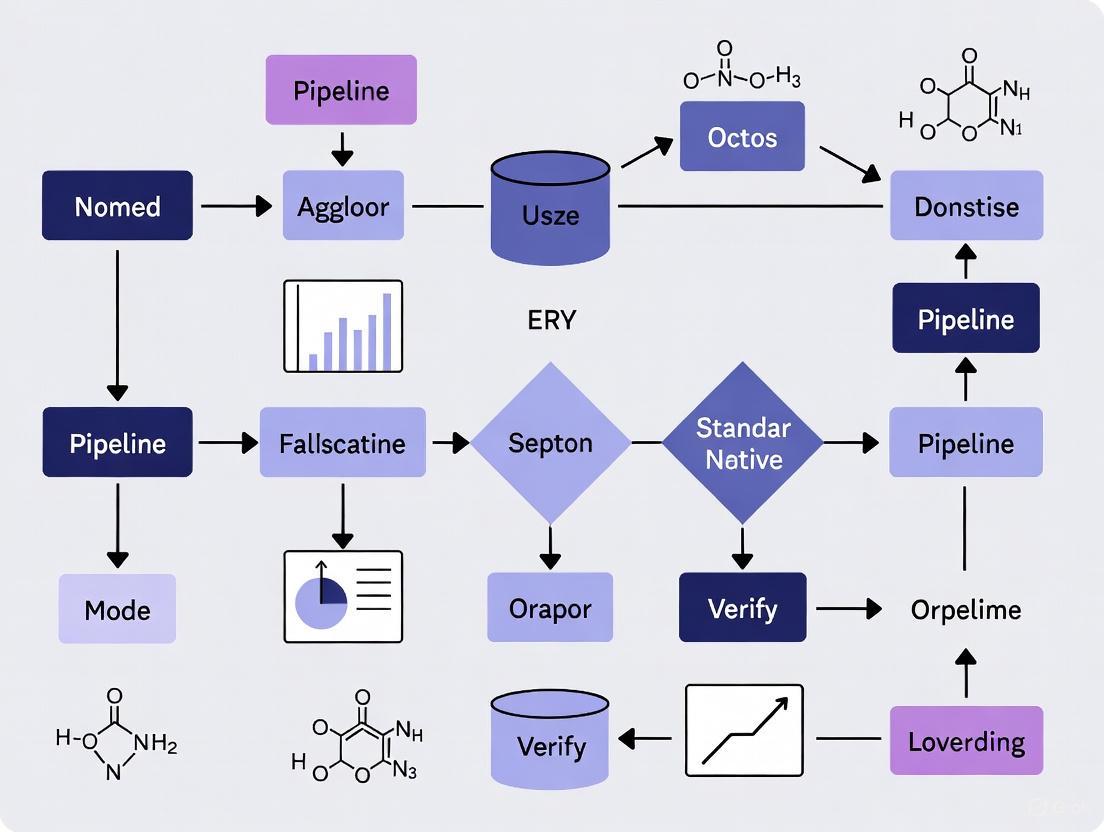
The Novel Organism Verification and Analysis (NOVA) pipeline is a specialized bioinformatics workflow designed for the detection and identification of bacterial isolates that cannot be characterized by conventional microbiological methods [3]. This pipeline was developed to address a critical gap in clinical bacteriology and research, where standard techniques like Matrix-Assisted Laser Desorption/Ionization Time-of-Flight Mass Spectrometry (MALDI-TOF MS) and partial 16S ribosomal RNA (rRNA) gene sequencing fail to identify novel or poorly characterized bacterial organisms [3] [16]. The implementation of NOVA provides researchers with a systematic approach for verifying novel taxa through whole genome sequencing (WGS), expanding our understanding of microbial diversity and enabling the discovery of potentially clinically relevant pathogens [3].

Table: NOVA Pipeline Performance in Identifying Novel Organisms

Metric	Result	Details
Total Isolates Analyzed	61	Isolates unidentifiable by conventional methods [3]
Novel Species Identified	35 (57%)	Representing potentially novel bacterial taxa [3]
Clinically Relevant Novel Strains	7	Isolated from deep tissue or blood cultures [3] [16]
Predominant Genera	Corynebacterium, Schaalia	Most frequently identified novel organisms [3]

Core Principles of the NOVA Pipeline

The NOVA pipeline operates on several fundamental principles that ensure its effectiveness in novel organism verification. First, it follows a hierarchical identification approach, where simpler, faster, and more cost-effective methods are employed initially, progressing to more complex genomic analyses only when necessary [3]. Second, it incorporates standardized verification thresholds, using clearly defined genetic similarity cutoffs (≤99.0% nucleotide identity in the 16S rRNA gene compared to described species) to determine when an isolate qualifies as a potential novel organism [3]. Third, the pipeline emphasizes data reproducibility and comparability through automated, standardized procedures that minimize manual intervention and subjective interpretation [17].

The operational framework of NOVA is designed to integrate seamlessly with routine diagnostic workflows while providing the specialized analytical capabilities required for novel organism characterization. The pipeline employs multiple verification methodologies including rMLST analysis, digital DNA-DNA hybridization (dDDH) with a 70% cutoff, and Average Nucleotide Identity (ANI) calculations to confirm the novelty of identified isolates [3]. This multi-faceted approach ensures robust taxonomic classification and provides researchers with comprehensive genomic evidence supporting the discovery of novel bacterial taxa.

Technical Specifications and Workflow

NOVA Pipeline Workflow

Decision Thresholds in the NOVA Pipeline

The NOVA pipeline employs specific, quantifiable thresholds to determine when an organism qualifies for novel species verification [3]:

Table: NOVA Pipeline Decision Thresholds

Analysis Stage	Threshold Criteria	Action Triggered
MALDI-TOF MS	Score < 2.0, divergent first/second hit results, or no validly published species match [3]	Proceed to 16S rRNA gene sequencing
16S rRNA Gene Sequencing	≤ 99.0% nucleotide identity (≥7 mismatches/gaps in analyzed sequence) [3]	Proceed to Whole Genome Sequencing
Whole Genome Sequencing	ANI index ≥ 96% between isolates [3]	Considered the same novel species
Digital DNA-DNA Hybridization	<70% similarity to known species [3]	Supports novel species designation

Essential Research Reagent Solutions

The successful implementation of the NOVA pipeline requires specific laboratory reagents, computational tools, and reference databases. The following table details the essential materials and their functions within the verification workflow:

Table: Research Reagent Solutions for NOVA Pipeline Implementation

Reagent/Resource	Function in Pipeline	Application Notes
EZ1 DNA Tissue Kit (Qiagen)	DNA extraction for WGS [3]	Ensures high-quality DNA for sequencing
Illumina Sequencing Platforms	Whole genome sequencing [3]	MiSeq or NextSeq500 systems used
Trimmomatic (v0.38)	Quality clipping of raw reads [3]	Pre-processing of sequencing data
Unicycler (v0.3.0b)	Genome assembly [3]	Creates assemblies from trimmed reads
Prokka (v1.13)	Genome annotation [3]	Automated annotation pipeline
TYGS Platform	Digital DDH analysis [3]	70% dDDH cutoff for species demarcation
OrthoANIu Algorithm	Average Nucleotide Identity calculation [3]	Determines genetic relatedness
NCBI RefSeq Database	Taxonomic classification [17]	Reference genome database
List of Prokaryotic Names with Standing in Nomenclature (LPSN)	Validation of novel species [3]	Determines "correctly described" species status

Frequently Asked Questions (FAQs)

Pipeline Implementation Questions

Q: What types of bacterial isolates should be submitted to the NOVA pipeline? A: The NOVA pipeline is specifically designed for isolates that cannot be reliably identified using conventional methods. This includes organisms with MALDI-TOF MS scores < 2.0, those showing divergent results between first and second hits, or those with no match to validly published species in standard databases [3]. The pipeline has proven particularly valuable for characterizing Gram-positive organisms, with Corynebacterium and Schaalia species being the most frequently identified novel taxa [3].

Q: What are the computational requirements for implementing the NOVA pipeline? A: While the original NOVA study utilized institutional computing resources, similar pipelines like ASA3P offer both local Docker container implementations for small-to-medium-scale projects and cloud computing versions for large-scale analyses [17]. The cloud version can automatically create and manage self-scaling compute clusters, enabling analysis of hundreds of bacterial genomes within hours [17].

Technical Troubleshooting Guide

Q: Our isolates pass the initial MALDI-TOF MS screening but fail during 16S rRNA sequencing. What could be causing this issue? A: This problem may stem from several sources:

• Primer specificity: Ensure that universal primers targeting approximately 800bp of the first part of the 16S rRNA gene are used [3]
• PCR inhibition: Check for inhibitors in your DNA extraction process; consider additional purification steps
• Database limitations: Verify that you're comparing sequences against the comprehensive NCBI 16S rRNA database using BLAST [3]
• Sequence quality: Implement quality control measures to ensure sequence accuracy before proceeding to WGS

Q: We have successfully sequenced a potential novel organism, but the bioinformatic analysis is yielding inconsistent taxonomic classifications. How should we proceed? A: The NOVA pipeline addresses this challenge through a multi-tool verification approach:

• Employ complementary methods: Use both rMLST and TYGS analysis concurrently [3]
• Apply stringent thresholds: Utilize the 70% dDDH cutoff and ANI calculations for consensus [3]
• Validate against type strains: Compare your isolates against all closely related type strains in public databases
• Manual curation: Examine conflicting results manually, focusing on genomic regions with discordant classifications

Data Interpretation and Validation

Q: How does the NOVA pipeline determine when an isolate represents a truly novel species rather than a strain of an existing species? A: The pipeline employs a hierarchical validation approach:

• Initial screening: ≤99.0% 16S rRNA gene sequence identity to described species [3]
• Genomic comparison: <95% ANI and <70% dDDH with closest known species [3]
• Multi-method consensus: Agreement across rMLST, TYGS, and OrthoANIu analyses [3]
• Validation against standards: Comparison with validly published species in LPSN [3]

Q: What evidence does the NOVA pipeline provide to support claims of novel species discovery? A: The pipeline generates comprehensive genomic evidence including:

• Complete genome assembly and annotation statistics [3]
• Comparative genomic metrics (ANI, dDDH) against closest known relatives [3]
• Taxonomic classification through multiple methods (rMLST, TYGS) [3]
• Documentation of genetic distinctiveness across the entire genome [3]

Advanced Methodological Protocols

Whole Genome Sequencing and Assembly Protocol

The WGS component of the NOVA pipeline follows a standardized protocol [3]:

• DNA Extraction: Use the EZ1 DNA Tissue Kit with EZ1 Advanced Instrument (Qiagen)
• Library Preparation: Utilize Illumina-compatible kits (NexteraXT or Illumina DNA prep)
• Sequencing: Perform on Illumina platforms (MiSeq or NextSeq500)
• Quality Control: Trim raw reads using Trimmomatic (v0.38)
• Genome Assembly: Create assemblies using Unicycler (v0.3.0b)
• Genome Annotation: Annotate using Prokka (v1.13)

Taxonomic Verification Protocol

For taxonomic verification of potential novel species [3]:

• rMLST Analysis: Perform ribosomal multilocus sequence typing for initial classification
• TYGS Analysis: Utilize the Type Strain Genome Server with 70% dDDH cutoff (method 2)
• ANI Calculation: Compute Average Nucleotide Identity using OrthoANIu algorithm
• Comparative Genomics: Compare against all closely related type strains in public databases
• Validation: Confirm novel status through consensus across all methods

This protocol ensures robust taxonomic classification and provides multiple lines of evidence supporting novel species designation, which is essential for publication and formal recognition of new bacterial taxa.

The identification of novel bacterial species in clinical settings presents a significant challenge for diagnosis and treatment. As research uncovers a vast diversity of previously uncharacterized pathogens, the limitations of conventional diagnostic methods become increasingly apparent. This technical support guide addresses the specific issues researchers and clinicians encounter when dealing with novel organisms, providing troubleshooting guidance and standardized protocols to enhance diagnostic accuracy and therapeutic development.

FAQs and Troubleshooting Guides

FAQ 1: What should I do when standard diagnostic methods fail to identify a bacterial isolate?

Answer: When conventional methods like MALDI-TOF MS and partial 16S rRNA gene sequencing fail to provide a reliable identification, implement a systematic verification pipeline.

• Problem: MALDI-TOF MS score is <2.0, results are divergent, or the species is not validly published [12] [3].
• Solution: Follow the Novel Organism Verification and Analysis (NOVA) algorithm [12] [3]:
  • Proceed to partial 16S rRNA gene sequencing (~800 bp).
  • Compare the sequence to the NCBI database using BLAST.
  • If the sequence has ≤99.0% nucleotide identity (≥7 mismatches/gaps) to any correctly described species, the isolate qualifies as a potentially novel species and should undergo Whole Genome Sequencing (WGS) [12] [3].

Troubleshooting Tip: A common point of failure is an incomplete reference database. Ensure you are using regularly updated databases like LPSN (List of Prokaryotic names with Standing in Nomenclature) to verify the taxonomic status of the closest match [12] [3].

FAQ 2: How do I determine if a newly identified species is clinically relevant?

Answer: Clinical relevance is determined through a collaborative assessment that integrates microbiological findings with patient clinical data.

An infectious disease specialist should evaluate the isolate based on these criteria [12] [3]:

• Clinical signs and symptoms compatible with an active infection.
• Presence of concomitant pathogens in the culture.
• Pathogenic potential of the bacterial genus to which the novel species belongs.
• Clinical plausibility of the isolate being the cause of the patient's condition.

Troubleshooting Tip: Monomicrobial growth from a normally sterile site (e.g., blood, deep tissue) significantly increases the likelihood of clinical relevance. In the NOVA study, 27 of 35 novel strains were isolated from deep tissue or blood cultures, and 7 were deemed clinically relevant [12] [3].

FAQ 3: Why does my 16S microbiome analysis give inconsistent species-level results, and how can I improve accuracy?

Answer: Inconsistencies often arise from the use of different variable regions, analysis pipelines, and reference databases, which lack standardization.

To improve accuracy [18] [19]:

• Target Region: For human gut microbiota, the V3-V4 regions are often used, but the V1-V2 region may provide better species differentiation [18] [19].
• Database: Use specialized, curated databases. A fixed 98.5% similarity threshold can cause misclassification; pipelines with flexible, species-specific thresholds (e.g., the asvtax pipeline) significantly improve precision [18].
• Methodology: Denoising techniques that produce Amplicon Sequence Variants (ASVs) offer single-nucleotide resolution but may be limited by poor database coverage of ASV diversity for many species [18].

Troubleshooting Tip: Validate your chosen pipeline and database against a set of well-characterized monobacterial samples to understand its limitations before applying it to complex clinical samples [19].

Experimental Protocols for Novel Species Identification

Protocol 1: The NOVA Study Whole Genome Sequencing Pipeline

This protocol is for the identification of bacterial isolates that cannot be characterized by conventional methods [12] [3].

1. DNA Extraction

• Reagent: EZ1 DNA Tissue Kit (Qiagen).
• Instrument: EZ1 Advanced Instrument (Qiagen).
• Function: Extracts high-quality genomic DNA for subsequent sequencing.

2. Whole Genome Sequencing

• Technology: Illumina (MiSeq or NextSeq500).
• Library Prep: NexteraXT or Illumina DNA prep kits.
• Function: Generates short-read sequence data for comprehensive genomic analysis.

3. Genome Assembly and Annotation

• Assembly Software: Unicycler v0.3.0b (assembles trimmed reads).
• Read Trimming: Trimmomatic v0.38.
• Annotation Software: Prokka v1.13.
• Function: Produces a complete genome assembly and identifies coding sequences.

4. Genomic Analysis for Classification

• Tools:
  • rMLST: For ribosomal multilocus sequence typing.
  • TYGS (Type (Strain) Genome Server): Uses a 70% digital DNA-DNA hybridization (dDDH) cutoff for species demarcation [12] [3].
  • Average Nucleotide Identity (ANI): Calculated using OrthoANIu. An ANI ≥96% with another strain indicates they belong to the same novel species [12] [3].

Protocol 2: Building a Specialized V3-V4 16S rRNA Database for Species-Level Identification

This protocol outlines the creation of a custom database to improve species-level classification of human gut microbiota from V3-V4 region sequencing [18].

1. Primary Database Construction

• Data Sources:
  • Seed sequences from LPSN and NCBI RefSeq databases.
  • 16S rRNA sequences from 1,082 human gut samples.
• Function: Creates a comprehensive foundation of trusted reference sequences.

2. Database Tailoring

• Target Region: Extract and focus on sequences from the V3-V4 regions (positions 341–806 of the 16S rRNA gene).
• Function: Creates a non-redundant Amplicon Sequence Variants (ASVs) database specific to the most commonly sequenced region.

3. Establish Flexible Thresholds

• Method: Analyze the database to determine genus- and species-specific classification thresholds, which can range from 80% to 100% similarity, moving beyond a fixed 98.5% cutoff.
• Function: Resolves misclassifications between closely related species and reduces false negatives.

4. Implement the asvtax Pipeline

• Method: Apply the flexible thresholds during taxonomic classification of new sequencing data.
• Function: Enhances the precision of species-level identification and improves the detection of new ASVs.

Data Presentation

Table 1: Outcomes of the NOVA Study Pipeline for Identifying Novel Bacterial Species [12] [3]

Category	Number of Isolates	Percentage	Notes
Total isolates in study	61	100%	Not identifiable by routine methods
Novel species	35	57%	Representing potentially new taxa
- Gram-positive	24	69%	Predominantly Corynebacterium and Schaalia
- Gram-negative	11	31%
- From deep tissue/blood	27	77%
- Clinically relevant	7	20%
Difficult-to-identify organisms	26	43%	Identifiable at species level only via WGS

Table 2: Key Research Reagent Solutions for Novel Organism Verification [12] [3]

Reagent / Kit	Function in the Protocol
EZ1 DNA Tissue Kit (Qiagen)	Extraction of high-quality genomic DNA from bacterial isolates.
NexteraXT / Illumina DNA Prep	Library preparation for Whole Genome Sequencing on Illumina platforms.
Trimmomatic v0.38	Quality trimming of raw sequencing reads prior to genome assembly.
Unicycler v0.3.0b	Hybrid assembly of sequencing reads into a complete genome.
Prokka v1.13	Rapid annotation of the assembled genome to identify coding sequences.

Workflow Visualization

The following diagram illustrates the decision pathway of the NOVA algorithm for identifying novel bacterial organisms in a clinical setting.

Decision Pathway for Novel Species Identification

Frequently Asked Questions

Q1: Our novel organism verification pipeline fails when comparing against biodiversity platforms like GBIF and OBIS. The error logs show "nomenclature mismatch" and "taxonomic conflict." How can we resolve this?

Inconsistent taxonomic naming between your internal database and global platforms is a common issue. Implement a taxonomic resolution service as an intermediate step in your pipeline. The NOVA study algorithm successfully handled this by using the List of Prokaryotic names with Standing in Nomenclature (LPSN) as an authoritative source to verify the "validly published" status of species names before cross-referencing [3]. Furthermore, global data initiatives are actively working on improving the interoperability between major platforms like OBIS and GBIF through shared standards and a consensus-based approach [20]. For your pipeline, you should:

• Integrate an automated step that checks species names against a curated nomenclatural database like LPSN or the Catalogue of Life (COL) [21] [3].
• Standardize your output using a common data standard like the Simple Knowledge Organization System (SKOS) to enhance future interoperability [22].
• Design your workflow to be "FAIR-by-design," ensuring data is Findable, Accessible, Interoperable, and Re-usable from the point of generation, as encouraged by European research initiatives [21].

Q2: We are unable to achieve species-level identification for many isolates using V3-V4 16S rRNA sequencing. What are the best practices to improve resolution for novel bacteria?

The limitation of the V3-V4 regions for species-level classification is a known challenge, but it can be addressed. Traditional fixed thresholds (e.g., 98.5-98.7% similarity) often cause misclassification because the actual 16S rRNA gene sequence divergence varies significantly between species [18]. A recent study developed a specialized pipeline that significantly improves resolution by creating a non-redundant Amplicon Sequence Variant (ASV) database and, most importantly, establishing flexible, species-specific classification thresholds instead of a single fixed cutoff [18]. To enhance your pipeline:

• Move beyond fixed thresholds. Develop or adopt a dynamic threshold system where the identity percentage for species classification is tailored to specific taxonomic groups [18].
• For the V3-V4 regions, consult databases that are specifically tailored to these sequences, as they provide more precise reference points than full-length 16S rRNA databases for this application [18].
• If high-resolution classification is critical, consider supplementing your analysis with Whole Genome Sequencing (WGS). The NOVA study demonstrated that WGS provides superior resolution when conventional methods like MALDI-TOF MS and 16S rRNA gene sequencing fail, using digital DNA:DNA hybridization (dDDH) and Average Nucleotide Identity (ANI) for definitive classification [3].

Q3: How can we assess the clinical relevance of a novel bacterial species identified by our pipeline?

Determining the clinical relevance of a novel organism requires a multi-faceted approach that combines genomic data with patient clinical information. The NOVA study established a protocol for this, where the clinical relevance of isolates representing novel species was evaluated retrospectively by an infectious disease specialist [3]. The assessment was based on several key criteria [3]:

• Patient Symptoms: The clinical signs and symptoms presented by the patient.
• Specimen Type: The anatomical source of the isolate (e.g., deep tissue or blood culture isolates are more likely to be significant).
• Culture Status: Whether the culture was monomicrobial or polymicrobial.
• Genus Potential: The known pathogenic potential of the bacterial genus.
• Clinical Plausibility: The overall plausibility that the isolate is causing the infection, considering all factors.

In their study, 7 out of 35 novel species were determined to be clinically relevant, with a majority isolated from deep tissue or blood cultures [3]. It is crucial to publicly share the clinical and genomic data of these novel organisms to help the broader scientific community better understand their ecological and clinical roles [3].

Q4: Our data pipeline struggles with integrating new data types, such as eDNA and morphological measurements. How can we structure this data for platforms like OBIS?

Global biodiversity data platforms are evolving to accommodate a wider variety of data beyond simple species occurrences. OBIS now supports the integration of contextual information through Extended Measurement or Fact (eMoF) data and other complementary data types [20]. To structure your data for successful integration:

• Adhere to the standardized formats required by the platform, such as the Darwin Core Archive standard, which can be extended for measurements and facts.
• For eDNA data, ensure you provide transparent metadata about the laboratory protocols, bioinformatics pipelines, and sequence quality control steps. OBIS highlights that new tools like eDNA require creative approaches for fast integration and seamless interoperability [20].
• Explicitly link species observations with associated habitat or environmental data to create context-enriched datasets that are significantly more valuable for ecological analysis and decision-making [20].

Experimental Protocols

Protocol 1: NOVA Algorithm for Novel Organism Verification and Analysis

This protocol is based on the NOVA (Novel Organism Verification and Analysis) study, designed for the systematic identification of bacterial isolates that cannot be characterized by conventional methods [3].

Workflow

The following diagram illustrates the key decision points and steps in the NOVA algorithm.

Materials and Reagents

Table 1: Key research reagents and materials for the NOVA pipeline [3].

Item Name	Function / Application	Specifications / Notes
Bruker MALDI-TOF MS	Initial rapid species identification using protein spectra.	Requires main spectra library database. Score ≥2.0 indicates reliable identification.
EZ1 DNA Tissue Kit (Qiagen)	Genomic DNA extraction from bacterial isolates.	Used on EZ1 Advanced Instrument for consistent yield.
Illumina DNA Prep Kit	Preparation of sequencing libraries for WGS.	Compatible with MiSeq or NextSeq500 platforms.
Trimmomatic (v0.38)	Bioinformatics tool for trimming adapter sequences and low-quality bases from raw sequencing reads.	Pre-processing step before genome assembly.
Unicycler (v0.3.0b)	Bioinformatics tool for bacterial genome assembly from short-read sequencing data.	Produces accurate assemblies for downstream analysis.
Prokka (v1.13)	Rapid annotation of prokaryotic genomes.	Identifies genes and other genomic features.
TYGS (Type (Strain) Genome Server)	Web-based platform for prokaryotic genome-based taxonomy and identification of novel species.	Uses a 70% digital DNA:DNA hybridization (dDDH) cutoff value.

Protocol 2: Building a Flexible Threshold Pipeline for 16S rRNA Species-Level Identification

This protocol is based on the study "A species-level identification pipeline for human gut microbiota based on the V3-V4 regions of 16S rRNA" [18].

Workflow

The following diagram outlines the process of constructing a specialized database and applying flexible thresholds for accurate species-level classification.

Materials and Reagents

Table 2: Key research reagents and materials for the flexible 16S rRNA pipeline [18].

Item Name	Function / Application	Specifications / Notes
SILVA, NCBI, LPSN Databases	Sources of high-quality, validated 16S rRNA reference sequences for primary database construction.	Used to build a foundational, non-redundant database.
Human Gut Samples (n=1,082)	Source of raw sequencing data to enrich the reference database with real-world Amplicon Sequence Variants (ASVs).	Improves coverage for strict anaerobes and uncultured organisms.
ASVtax Pipeline	A specialized bioinformatics tool for taxonomic classification that applies flexible, species-specific identity thresholds.	Resolves misclassification between closely related species and reduces false negatives.
k-mer Feature Extraction	A bioinformatics method used within the pipeline to compare sequence similarity based on short subsequences of length k.	Helps in precise annotation of new ASVs.
Probabilistic Models	Statistical models used to support taxonomic assignment based on sequence data and defined thresholds.	Increases the reliability of the classification output.

Table 3: Major biodiversity data platforms and their primary functions relevant to taxonomic research [20] [23].

Platform Name	Primary Function	Data Type / Focus
GBIF	Global database for species occurrence data.	Terrestrial and marine species distribution records.
OBIS	Global database for marine biodiversity data.	Ocean species observations, biogeochemistry, and eDNA.
Catalogue of Life (COL)	Authoritative global taxonomy for known species.	Standardized species names and hierarchical classification.
LPSN	List of Prokaryotic names with Standing in Nomenclature.	Validly published names for bacteria and archaea.
ENCORE	Tool for understanding ecosystem dependencies and impacts.	Helps financial institutions screen portfolio risks.
IBAT	Provides access to IUCN Red List and protected areas data.	Site-level risk screening for conservation planning.

Implementing a Robust Verification Pipeline: From Sample to Genome Assembly

The NOVA Algorithm represents a structured methodology for enhancing the reliability and reproducibility of analyses within novel organism verification pipelines. In the critical field of drug development, where research on non-model organisms is increasingly prevalent, standardizing the verification process is paramount. This technical support center provides researchers, scientists, and development professionals with essential troubleshooting guides and frequently asked questions to facilitate the successful implementation of the NOVA Algorithm in their experimental workflows. The guidance below is framed within the context of creating a robust, standardized approach to verifying novel organisms for biomedical research.

Frequently Asked Questions (FAQs)

Q1: What is the core purpose of the NOVA Algorithm in a verification pipeline? The NOVA Algorithm provides a structured, iterative planning and search framework designed to enhance the novelty and diversity of outputs while ensuring systematic and reliable analysis. In organism verification, it helps plan the acquisition of external knowledge (e.g., genomic databases, literature) to progressively enrich the analysis and avoid repetitive or simplistic conclusions [24]. It is based on a suite of practical alignment techniques that have been empirically validated to produce high-performing, reliable models [25].

Q2: During the initial seed generation phase, my results lack diversity. What could be the issue? A lack of diversity in initial seeds typically stems from a constrained knowledge base. The NOVA framework initiates with a multi-source seed generation module that activates using diverse inputs and scientific discovery techniques [24].

• Solution: Ensure your input is rich and contextual. Combine the target organism's data with directly referenced or related studies to fully understand the current landscape, including established methods, innovations, and, crucially, recognized weaknesses and limitations [24]. This comprehensive understanding is the foundation for generating varied and novel hypotheses.

Q3: How does the iterative refinement phase in NOVA improve the verification analysis? The iterative refinement phase addresses the problem of repetitive outputs by purposely planning the retrieval of external knowledge. Instead of undirected searches, the model devises a plan in each iteration to find information that will specifically enhance the novelty and diversity of the current analysis [24]. This targeted approach leads to a substantial increase in unique and high-quality outputs, with studies showing the number of unique novel ideas can be 3.4 times higher than approaches without such a framework [24].

Q4: What are the best practices for ensuring the reliability of individual analysis steps? The NOVA philosophy emphasizes breaking down complex workflows into reliable, atomic commands. Focus on achieving high reliability (e.g., >90% accuracy in internal evaluations) on fundamental capabilities before composing them into more complex workflows [26]. This ensures that each step in your verification protocol, from data retrieval to a specific analysis, is a dependable building block.

Q5: Are there specific customization options for the NOVA Algorithm in biological verification? Yes, the underlying NOVA models support extensive customization through a comprehensive suite of fine-tuning capabilities. Researchers can fine-tune the models on their proprietary data—including unique genomic datasets and organism-specific characteristics—to generate fully customized outputs that align with specific verification requirements and style guidelines [27].

Troubleshooting Guides

Issue 1: Low Success Rate in Automated Knowledge Retrieval

Problem: The automated system fails to retrieve relevant or high-quality external data during the iterative planning phase.

Diagnosis:

• The search plan may be too vague or not goal-oriented.
• The data sources may not be adequately integrated or accessible.

Resolution:

• Refine the Search Plan: Instruct the model to create more specific plans. Instead of "find related papers," the prompt should be "search for papers published in the last two years detailing the metabolic pathways of [Genus] and their known secondary metabolites."
• Validate Data Sources: Ensure integration with authoritative biological databases (e.g., NCBI, UniProt) and that API endpoints are functional. The system should be able to interact with these external environments dynamically [24].

Issue 2: Inconsistent or Non-Reproducible Results Between Runs

Problem: Executing the same NOVA workflow with identical input parameters yields significantly different results.

Diagnosis:

• This is often due to non-determinism in model sampling or variations in the live data retrieved from external sources.

Resolution:

• Parameter Tuning: During the fine-tuning and optimization phase, employ a consistent random seed. For training, models in the NOVA suite often use a learning rate of 1e-5 over 2-6 epochs with sample packing and weight decay to prevent overfitting [25].
• Snapshot Databases: For reproducibility, use versioned or snapshotted database downloads for critical reference data, rather than live queries, during the development and validation of your pipeline.

Issue 3: Inadequate Contrast in Generated Workflow Visualizations

Problem: Diagrams generated for signaling pathways or experimental workflows are difficult to read due to poor color contrast, making them inaccessible.

Diagnosis:

• The visualization tool has not enforced sufficient contrast between foreground elements (text, lines) and their backgrounds.

Resolution:

• Enforce Contrast Rules: Implement a color contrast analyzer to ensure all visual elements meet the WCAG enhanced contrast requirement of at least a 4.5:1 ratio for large text and 7:1 for other text [28] [29].
• Use Approved Palette: Restrict your visualization color palette to the following and explicitly set fontcolor for high contrast against the node's fillcolor:
  • #4285F4, #EA4335, #FBBC05, #34A853, #FFFFFF, #F1F3F4, #202124, #5F6368

For example, a node with a fillcolor="#4285F4" (blue) should have fontcolor="#FFFFFF" (white) for optimal readability.

Experimental Protocols & Data

Quantitative Performance Data

The following table summarizes the core performance improvements observed from the application of NOVA alignment techniques on established base models, demonstrating its effectiveness in enhancing model capabilities for complex tasks [25].

Table 1: Model Performance Enhancement with NOVA Alignment

Model Variant	Benchmark	Base Model Score	NOVA-Aligned Score	Relative Improvement
Qwen2-Nova-72B	User Experience (Overall)	Baseline	-	17% - 28%
Qwen2-Nova-72B	User Experience (Mathematics)	Baseline	-	28%
Qwen2-Nova-72B	User Experience (Reasoning)	Baseline	-	23%
Llama3-PBM-Nova-70B	ArenaHard Benchmark	46.6	74.5	~60%

Detailed Methodology: Iterative Planning and Search

This protocol is adapted from the Nova pipeline for enhancing novelty in research ideas and can be applied to generating novel hypotheses in organism verification [24].

1. Initial Seed Generation:

• Input: Primary data for the target organism (e.g., raw genomic sequence).
• Prompting: Use a structured prompt template to guide the model. The prompt should assign a role (e.g., "expert bioinformatician"), outline the steps for understanding the input data and its context (e.g., related organisms), and require the identification of tasks, methods, innovations, and weaknesses.
• Output: A set of initial, multi-source seed ideas or hypotheses for verification.

2. Iterative Refinement:

• Planning: For each seed idea, task the model with creating a "search plan." This plan should specify what new knowledge is needed to make the hypothesis more novel or robust (e.g., "Find papers on virulence factors in closely related bacterial species").
• Search Execution: Execute the search plan by querying integrated external databases and literature repositories.
• Knowledge Integration: Feed the retrieved knowledge back to the model and prompt it to refine the original seed idea.
• Repeat: Conduct multiple iterations of planning and searching to progressively broaden and deepen the analysis.

3. Detailed Completion:

• The final stage involves using the refined and enriched ideas to generate a complete and detailed analysis report or verification outcome.

Workflow Visualization

The following diagram illustrates the core NOVA Algorithm workflow for systematic analysis, depicting the stages from input to final output and the critical iterative refinement loop.

The Scientist's Toolkit: Research Reagent Solutions

Table 2: Essential Reagents and Materials for a NOVA-Aligned Verification Pipeline

Item / Solution	Function in the NOVA Workflow	Example/Note
High-Quality Genomic DNA Kit	Provides the primary input data ("Target Paper") for the verification analysis.	Essential for generating reliable sequencing data as the foundational input.
Multi-Source Reference Databases	Serves as the "Referenced Papers" for contextual understanding and iterative knowledge retrieval.	Integrate NCBI, UniProt, and specialized organism databases via API.
NOVA-Aligned Foundation Model	The core engine for executing the algorithm's planning, search, and generation steps.	Can be accessed via APIs (e.g., Amazon Bedrock) and fine-tuned on proprietary data [27] [25].
Custom Fine-Tuning Dataset	Allows adaptation of the base model to reflect specific industry expertise and verification goals.	A curated dataset of proprietary genomic annotations and verification reports [27].
Automated Planning & Search SDK	Provides the building blocks to break down complex verification workflows into reliable, atomic commands.	The Amazon Nova Act SDK enables the creation of agents that can automate browser-based data retrieval tasks [26].

Specimen Processing and Culture Conditions for Diverse Bacterial Isolates

This technical support guide outlines standardized protocols for the processing and cultivation of diverse bacterial isolates, a critical component of a novel organism verification pipeline. The methods detailed herein are designed to ensure reproducibility, minimize contamination, and maximize the recovery of target organisms for downstream research and drug development applications. A core principle across all procedures is the critical distinction between sterilization, which eliminates all microorganisms, and disinfection, which reduces the microbial population to a safe level [30]. Adherence to these protocols is fundamental to obtaining pure cultures and reliable, interpretable results.

Frequently Asked Questions (FAQs) and Troubleshooting

Q1: My culture plates show no growth after incubation. What are the primary causes?

• Incorrect Culture Conditions: Verify that the temperature, atmosphere (aerobic, anaerobic, microaerophilic), and pH of the medium are appropriate for your target bacterium. For example, anaerobic bacteria will not grow in ambient air without special equipment like an anaerobic chamber [31] [32].
• Improper Sample Processing: The sample may contain viable but non-culturable cells, or the processing method (e.g., excessive heating, harsh chemical treatment) may have killed the bacteria.
• Nutrient Deficiency: The culture medium may lack a specific nutrient, vitamin, or growth factor required by the bacterium. For instance, lactobacilli require supplemented vitamins [30].
• Incorrect Medium pH: The pH of the medium might be unsuitable. Bacteria generally prefer a neutral to slightly alkaline pH, while molds prefer an acidic environment [30].

Q2: How can I prevent contamination during specimen processing and culture?

• Aseptic Technique: Always perform work near a Bunsen burner flame or in a laminar flow cabinet to create a sterile field. Sterilize all instruments, such as inoculation loops and needles, by flaming before and after use [30].
• Proper Sterilization: Ensure all media, reagents, and labware (e.g., petri dishes, pipettes, solutions) are sterilized using an validated autoclave cycle (typically 121°C for 15-30 minutes) [30].
• Control Measures: Include negative controls (e.g., uninoculated media) in every experiment. If contamination is found in these controls, it indicates a failure in media sterilization or aseptic technique [30].

Q3: My mixed culture is not separating into distinct colonies. How can I improve isolation?

• Refine Streaking Technique: Use the quadrant streak method on a solid agar plate. Ensure you flame and cool the loop between each quadrant to progressively dilute the bacterial load, which is crucial for obtaining single colonies [30] [32].
• Optimize Dilution: If using the spread-plate method, ensure the bacterial suspension is sufficiently diluted. Try several log-fold dilutions to achieve a concentration where individual cells are physically separated on the agar surface [32].
• Use Selective Media: Incorporate selective agents (e.g., antibiotics, specific carbon/nitrogen sources, high salt) into the agar to inhibit the growth of unwanted microbes and favor the growth of your target isolate [30].

Q4: How should I handle and preserve isolated bacterial strains for long-term study?

• Short-Term Storage: For strains in active use, pure cultures can be stored on agar slants at 4°C for several weeks. However, this method is prone to genetic variation and contamination over time [30].
• Long-Term Preservation: For stable, long-term storage, the glycerol stock method is recommended. Suspend a fresh bacterial culture in a cryoprotectant like 20-50% sterile glycerol broth, then store at -80°C. This method preserves viability for years [31] [30].

Experimental Protocols for Isolation and Identification

Standard Workflow for Specimen Processing and Pure Culture Isolation

The following protocol provides a generalized workflow for processing complex samples to obtain pure bacterial cultures.

Materials & Reagents:

• Sample: Water, soil, or clinical specimen.
• Buffers: Phosphate-Buffered Saline (PBS) or physiological saline (0.85-0.9% NaCl).
• Culture Media: Non-selective broth (e.g., LB, TSB), solid agar plates (general purpose like R2A or nutrient agar), and selective agar as needed [33] [30].
• Equipment: Sterile tubes, pipettes, spreaders, inoculation loops, incubator, centrifuge, and biosafety cabinet.

Procedure:

• Sample Homogenization:
  • Liquid samples: Vortex and serially dilute in sterile diluent (e.g., PBS or saline) [33].
  • Solid samples (e.g., soil, tissue): Aseptically weigh a portion, add to diluent with sterile glass beads, and vortex vigorously to create a homogeneous suspension [33].
• Inoculation and Incubation:
  • Spread-Plate Method: Spread 50-100 µL of an appropriate sample dilution onto solid agar plates and incubate under suitable conditions until colonies appear (typically 24-72 hours) [33] [32].
  • Streak-Plate Method: Using a sterile loop, streak the sample or a colony from a spread-plate onto a fresh agar plate to isolate single colonies [30] [32].
• Colony Selection and Purification:
  • Examine plates for colonies of differing morphology (shape, color, size, edge).
  • Sub-culture each distinct colony type onto a fresh agar plate by streaking to ensure purity. Repeat if necessary until a pure culture is obtained [33] [32].

Bacterial Identification via MALDI-TOF Mass Spectrometry

Matrix-Assisted Laser Desorption/Ionization Time-of-Flight (MALDI-TOF MS) provides rapid, high-throughput species identification based on protein mass fingerprints [34] [31].

Materials & Reagents:

• Target Plate: 384-spot steel MALDI target plate.
• Matrix Solution: Saturated α-cyano-4-hydroxycinnamic acid (CHCA) in 50% acetonitrile and 2.5% trifluoroacetic acid.
• Calibration Standard: Commercial peptide or protein standard for the mass spectrometer.
• Ethanol and Formic Acid.

Procedure:

• Sample Preparation: Smear a small amount of a fresh bacterial colony directly onto a target plate spot. Overlay with 1 µL of 70% formic acid and allow to air dry.
• Matrix Application: Cover the dried sample spot with 1 µL of the saturated CHCA matrix solution and allow it to crystallize at room temperature [34].
• Instrument Analysis: Insert the target plate into the MALDI-TOF MS instrument. Acquire spectra in positive linear ion mode across a mass range of 2,000 to 20,000 Da, using the calibration standard for accuracy [34].
• Data Interpretation: Compare the acquired protein mass fingerprint (peak list) against a reference database. A score of ≥ 9 is typically considered a confident species-level identification [31].

Data Presentation and Workflow Visualization

Quantitative Data Table: Common Selective Media Components

The table below summarizes key components of selective media and their applications for isolating specific bacterial types.

Table: Selective Media Components and Applications

Media Component	Concentration/Type	Function & Target Microorganisms
Sodium Chloride (NaCl)	5-25% (w/v)	Selects for halotolerant and halophilic bacteria (e.g., Staphylococcus aureus, marine bacteria) [33] [30].
Antibiotics	Varies (e.g., Chloramphenicol)	Inhibits a broad range of bacteria, allowing for the isolation of fungi and antibiotic-resistant bacteria [30].
Specific Carbon Source	Cellulose, Petroleum, Urea	Enriches for bacteria with specific metabolic capabilities (e.g., cellulose degraders, hydrocarbon degraders, urease producers) [30].
Bile Salts	Varies	Inhibits gram-positive bacteria, selects for gram-negative enteric bacteria [30].

Research Reagent Solutions

Table: Essential Reagents for Bacterial Processing and Identification

Reagent/Kit	Function/Application
Glycerol (50% v/v, sterile)	Cryoprotectant for long-term storage of bacterial isolates at -80°C [31] [30].
C18 Solid-Phase Extraction Columns	Purification and desalting of peptide mixtures for downstream analysis like ZooMS or LC-MS [34].
DNeasy Blood & Tissue Kit	Extraction of high-quality genomic DNA for downstream applications such as 16S rRNA gene sequencing or whole-genome sequencing [31].
Trypsin	Protease enzyme for digesting proteins into peptides for mass spectrometric fingerprinting (e.g., ZooMS, proteomics) [34].
CHCA Matrix	Organic matrix compound for co-crystallization with analyte in MALDI-TOF MS [34].
16S rRNA PCR Primers (27F, 1492R)	Amplification of the 16S rRNA gene for Sanger sequencing and phylogenetic identification of bacteria [31].

Workflow and Troubleshooting Diagrams

Diagram: Specimen Processing for Pure Cultures

Diagram: Troubleshooting No Bacterial Growth

Troubleshooting Guide: Addressing Common WGS Experimental Challenges

This guide provides solutions for specific, data-quality issues that can arise during Whole Genome Sequencing experiments, particularly within novel organism verification pipelines.

TABLE: Whole-Genome Sequencing Troubleshooting Guide

Problem Identification	Possible Cause	Recommended Solution
Failed reactions with messy traces and mostly N's in the data [35].	Low template DNA concentration, poor DNA quality, or excessive template DNA [35].	Confirm DNA concentration is 100-200 ng/µL using a precise method (e.g., NanoDrop). Ensure high-quality DNA (OD 260/280 ≥ 1.8) and use a cleanup kit to remove contaminants [35].
High background noise along the trace baseline, leading to low-quality scores [35].	Low signal intensity due to poor amplification from low template concentration or inefficient primer binding [35].	Re-check and adjust template concentration. Verify primer quality, ensure it is not degraded, and confirm high binding efficiency [35].
Sequence termination or drastic signal drop after a region of good quality data [35].	Secondary structures (e.g., hairpins) or long homopolymer stretches (e.g., polyG, polyC) that the polymerase cannot traverse [35].	Use an alternate sequencing chemistry designed for difficult templates (e.g., ABI's "difficult template" protocol). Alternatively, design a new primer that binds after the problematic region [35].
"Double sequence" or mixed peaks starting partway through an otherwise high-quality trace [35].	Colony contamination (sequencing multiple clones) or the presence of a toxic sequence in the DNA causing rearrangements in E. coli [35].	Ensure a single colony is picked for sequencing. For toxic sequences, use a low-copy vector, grow cells at 30°C, and avoid overgrowth [35].
Poorly resolved, broad peaks instead of sharp, distinct peaks [35].	Potential unknown contaminant in the DNA sample or, rarely, degraded polymer in the sequencer [35].	Use a different DNA cleanup method or dilute the template. The sequencing facility will typically re-run samples if an instrument issue is suspected [35].

Frequently Asked Questions (FAQs)

Q1: What are the primary advantages of Whole Genome Sequencing over targeted approaches? WGS provides a comprehensive, high-resolution, base-by-base view of the entire genome. This allows it to capture a wide range of variants—including single nucleotide variants, insertions/deletions, copy number changes, and large structural variants—that might be missed with targeted methods like exome sequencing. It is ideal for discovery applications, such as novel genome assembly and identifying novel causative variants [36].

Q2: When should Ultra-Rapid Whole Genome Sequencing be considered? Ultra-Rapid WGS is critical for time-sensitive clinical scenarios where a rapid genetic diagnosis could directly impact medical management and outcomes. Indications include [37]:

• Critically ill infants in intensive care with no unifying diagnosis.
• Primary admission for intractable seizures.
• Unexplained cardiac arrest.
• Situations where invasive procedures (e.g., biopsies) may be avoided with a genetic diagnosis.

Q3: What are the key specimen requirements for successful WGS? Whole blood collected in an EDTA tube is the most common and validated specimen. DNA isolated from such blood is also acceptable. Saliva specimens may be used for supplementary analysis like phasing. Template DNA concentration must be accurately measured and ideally fall between 100 ng/µL and 200 ng/µL for optimal results [35] [37].

Q4: How should I submit my genome assembly and associated data to a public repository? You can submit your genome assembly to GenBank and choose to hold it until your paper's publication. The primary reads used for assembly should be submitted to the Sequence Read Archive (SRA). It is crucial to register a BioProject for your research effort and a separate BioSample for each genome specimen. The assembled genome can be submitted with or without annotation [38].

Q5: What categories of genomic variation can a validated WGS pipeline detect? A clinically validated WGS pipeline is typically capable of reporting on [37]:

• Single nucleotide variants (SNVs)
• Small insertions and deletions (Indels)
• Small and large copy number variations (CNVs)
• Aneuploidy (whole chromosome)
• Mitochondrial DNA variants
• Gene-specific copy number analysis (e.g., SMN1/SMN2)

Experimental Protocol: Comprehensive WGS for Novel Organisms

This protocol outlines a detailed methodology for whole genome sequencing of a novel organism, from sample preparation to data submission, supporting standardized verification pipelines.

1. Sample Collection and DNA Extraction:

• Collect biomass from the novel organism using sterile techniques to avoid contamination.
• Perform DNA extraction using a kit optimized for your sample type (e.g., microbial, plant, fungal). The goal is to obtain high-molecular-weight DNA.
• Assess DNA purity by spectrophotometry (A260/A280 ratio of ~1.8 and A260/A230 > 2.0) and integrity by agarose gel electrophoresis (a single, tight high-molecular-weight band).

2. DNA Quantification and Quality Control:

• Quantify the DNA accurately using a fluorescence-based method (e.g., Qubit) as it is more specific for double-stranded DNA than spectrophotometry.
• Precisely dilute the DNA to the required concentration for your library prep kit (often within the 100-200 ng/µL range [35]).

3. Library Preparation and Sequencing:

• Fragment the genomic DNA to the desired size (e.g., 350-550 bp) using acoustic shearing or enzymatic fragmentation.
• Perform end-repair, A-tailing, and adapter ligation using a commercial library preparation kit. Include dual-index barcodes to multiplex samples.
• Perform library quantification and quality control via qPCR and fragment analysis (e.g., Bioanalyzer).
• Sequence the library on an appropriate next-generation sequencing platform (e.g., Illumina NovaSeq for high coverage) using a paired-end strategy (e.g., 2x150 bp). For novel organisms, aim for a high sequencing depth (>50x coverage).

4. Data Analysis and Genome Assembly:

• Perform primary analysis (base calling and demultiplexing) on the instrument's output.
• Run secondary analysis: perform quality control on raw reads (using FastQC), adapter trimming, and error correction.
• For de novo assembly, use an assembler like SPAdes (for microbial genomes) or CANU (for long-read data) to construct contigs and scaffolds from the cleaned reads.
• Assess assembly quality using metrics like N50, number of contigs, and completeness (using tools like BUSCO).

5. Data Submission:

• Submit the raw sequencing reads to the Sequence Read Archive (SRA).
• Submit the final assembled genome to GenBank. You will need the associated BioProject and BioSample accessions. Annotation can be submitted as a 5-column feature table (.tbl) file [38].

Workflow Visualization: WGS for Novel Organisms

WGS Pipeline for Novel Organisms

The Scientist's Toolkit: Essential Research Reagents & Materials

TABLE: Key Reagents for Whole Genome Sequencing

Item	Function
High-Fidelity DNA Polymerase	Essential for accurate amplification during library preparation, minimizing errors in the sequenced fragments.
Library Preparation Kit	A commercial kit containing all necessary enzymes and buffers for end-repair, A-tailing, adapter ligation, and library amplification.
Indexed Adapters	Short, double-stranded DNA sequences containing sequencing primer binding sites and unique molecular barcodes to multiplex multiple samples in a single run.
Size Selection Beads	Magnetic beads (e.g., SPRI beads) used to purify and select for DNA fragments within a specific size range after shearing and library prep.
Quality Control Assays	Kits and reagents for quantifying (e.g., Qubit dsDNA HS Assay) and qualifying (e.g., Bioanalyzer High Sensitivity DNA kit) the library before sequencing.
Reference Genome Sequence	A known genomic sequence from a closely related organism, used as a guide for read alignment during resequencing projects. Not needed for de novo assembly.

The identification and characterization of novel bacterial species from clinical and environmental samples are crucial for advancing microbiology and therapeutic development. Conventional identification methods, such as MALDI-TOF MS and partial 16S rRNA gene sequencing, frequently fail to characterize novel organisms due to insufficient reference data. The Novel Organism Verification and Analysis (NOVA) study demonstrated that whole-genome sequencing (WGS) provides the necessary resolution, successfully identifying 35 clinical isolates representing potentially novel bacterial taxa that evaded conventional methods [3]. Such research highlights the critical need for standardized, reproducible bioinformatics pipelines in novel organism verification.

Hybrid genome assembly and automated annotation form the cornerstone of modern genomic analysis. Within this context, two tools have become essential: Unicycler for hybrid assembly of bacterial genomes, and Prokka for rapid genome annotation [39]. The integration of these tools into robust pipelines enables researchers to efficiently transition from raw sequencing reads to a fully annotated genome, a process fundamental to understanding an organism's genetic makeup and pathogenic potential. This technical support center addresses common challenges and provides optimized protocols to ensure the reliability of these analyses within a standardized verification framework.

Unicycler is a specialized hybrid assembly pipeline for bacterial genomes. It integrates both short-read (e.g., Illumina) and long-read (e.g., Oxford Nanopore, PacBio) data to produce high-quality assemblies. Unicycler employs a short-read-first approach, using SPAdes for initial assembly and then leveraging long reads to scaffold and resolve repeats, which is particularly effective with lower-depth or lower-accuracy long reads [40]. Its key outputs include a FASTA file of contigs and an assembly graph for visualization in tools like Bandage [41] [40].

Prokka is a command-line software tool for the rapid annotation of prokaryotic genomes. It automates the process of identifying genomic features—such as protein-coding genes (CDS), ribosomal RNA, and tRNA genes—by leveraging multiple prediction tools (e.g., Prodigal for CDS, RNAmmer for rRNA) and produces standards-compliant output files (e.g., GFF3, GenBank format) suitable for submission to public databases [42] [39].

The following workflow illustrates how these tools integrate into a complete genome analysis pipeline for novel organism verification:

Figure 1: Standard workflow for bacterial genome assembly and annotation, incorporating quality control and evaluation steps.

Unicycler Assembly Troubleshooting Guide

Frequently Asked Questions

Q: My Unicycler hybrid assembly fails with a segmentation fault. What should I do? A: Segmentation faults can stem from various issues. First, try rerunning the job as it might be a transient cluster issue [43]. If it persists, perform rigorous quality control on your reads using FastQC and apply trimming with tools like Trimmomatic to remove adapters and low-quality bases. The presence of sequencing artifacts or contamination can cause assembly failures [43].

Q: How can I tell if my bacterial genome assembly is complete? A: A complete bacterial assembly has each chromosome and plasmid represented by a single, circular contig. Examine the Unicycler log file for a summary of graph components. It will indicate if components are circular. Furthermore, you can visualize the assembly graph (assembly.gfa) in Bandage. In a complete assembly, each replicon will appear as a single circle [41].

Q: My assembly is incomplete. What manual completion strategies can I try? A: If Unicycler produces an incomplete, tangled graph, several investigative approaches can help:

• Use Bandage to visualize assembly graphs from different stages of the Unicycler pipeline [41].
• Extract long reads that map to the incomplete regions and BLAST them to the graphs to find connections [41].
• Align both short and long reads to the assembly and examine the alignments in IGV or Artemis to identify misassemblies or gaps [41].
• Try assembling the reads with a different long-read assembler like Canu and compare the results to Unicycler's assembly [41].

Q: Should I use Unicycler for all my bacterial genome assemblies? A: Unicycler excels at short-read-first hybrid assembly, making it ideal when long-read depth is low. However, if you have high-depth, high-accuracy long reads (common with modern Nanopore sequencing), a long-read-first approach using tools like Trycycler followed by short-read polishing with Polypolish may yield superior results [40].

Common Unicycler Errors and Solutions

Table 1: Troubleshooting common Unicycler assembly problems.

Error or Problem	Potential Cause	Solution
Segmentation fault [43]	Transient cluster error, poor read quality, or problematic data.	Rerun the job; perform QC and trimming with FastQC/Trimmomatic [43].
Incomplete assembly with tangled graph [41]	Genuine biological complexities (repeats) or insufficient long-read coverage.	Use Bandage for visualization and manual investigation; gather more long reads for weak spots [41].
Unicycler fails to use long reads effectively	Large genome or highly complex repeats.	Verify long read quality and quantity; consider a long-read-first assembler like Trycycler for high-quality long reads [40].
High misassembly rate	Incorrect repeat resolution.	Use the --conservative mode to favor fewer misassemblies over contiguity; check reads with IGV/Artemis [40].

Unicycler Quick Start Protocol

Command-Line Protocol: Hybrid Genome Assembly with Unicycler

Objective: Assemble a bacterial genome from Illumina paired-end reads and Oxford Nanopore long reads.

Input Data:

• short_reads_1.fastq.gz: Illumina forward reads.
• short_reads_2.fastq.gz: Illumina reverse reads.
• long_reads.fastq.gz: Oxford Nanopore reads.

Method:

• Basic Hybrid Assembly Command:
  This command will run Unicycler with default parameters, which is suitable for most use cases [40].

• Key Parameters for Troubleshooting:

  • --mode: Choose assembly mode. Use --mode conservative to reduce misassemblies (may result in a more fragmented assembly) [43].
  • --min_fasta_length: Set a minimum contig length (default: 100 bp).
  • --linear_seqs: Specify the number of expected linear sequences (e.g., chromosomes/plasmids), if known.

• Output Analysis:

  • The primary assembly will be in output_dir/assembly.fasta.
  • The assembly graph for visualization in Bandage is output_dir/assembly.gfa.
  • Inspect the output_dir/unicycler.log for a summary of the assembly process and completion statistics [41].

Prokka Annotation Troubleshooting Guide

Frequently Asked Questions

Q: Prokka does not assign gene names (e.g., "lpxC") to my features, only product names. How can I fix this? A: This is expected default behavior. Prokka outputs the product information (e.g., "Lipid A biosynthesis myristoyltransferase") in the FASTA files by default. To include the gene name, you must use the --addgenes flag. This option adds a gene tag to the annotation from the protein database search. Note that the gene name will be visible in the GFF and GenBank output files, but the FASTA headers will still primarily show the product [44].

Q: How can I improve annotation quality for a novel organism with no close reference in databases? A: For novel organisms, follow these steps:

• Use the best available reference: Provide Prokka with protein sequences from the closest available relative using the --proteins option [42] [44].
• Adjust e-value threshold: Loosen the e-value cutoff (e.g., --evalue 1e-6) for distant homology searches [42].
• Leverage RNA-seq data: If available, use transcriptomic evidence to guide and validate gene models, though this is more common in eukaryotic annotation [45].
• Verify gene predictions: Use tools like BUSCO to assess annotation completeness against conserved single-copy orthologs [45].

Q: I am preparing a genome for submission to NCBI or ENA. What Prokka settings should I use? A: Use the --compliant flag to enforce Genbank/ENA/DDJB formatting rules. This option automatically enables --addgenes, sets --mincontiglen to 200, and requires you to specify a sequencing centre using --centre. You must also register your locus_tag prefix with NCBI/ENA beforehand and specify it using --locustag [42].

Q: Can Prokka annotate archaeal or viral genomes? A: Yes. Use the --kingdom parameter to change the annotation mode: --kingdom Archaea for archaea or --kingdom Viruses for viruses. This adjusts the underlying genetic code and prediction parameters [42].

Prokka Annotation Output Files

Table 2: Key output files generated by Prokka and their descriptions.

File Extension	Description
.gff	The master annotation in GFF3 format, containing both sequences and annotations. Viewable in Artemis or IGV [42].
.gbk	A standard GenBank file format derived from the master .gff file [42].
.faa	Protein FASTA file of the translated CDS sequences [42].
.ffn	Nucleotide FASTA file of all predicted transcripts (CDS, rRNA, tRNA, etc.) [42].
.tsv	Tab-separated file of all features with columns for locus_tag, gene, product, and other annotations [42].
.err	The NCBI discrepancy report, listing annotations that may be problematic for submission [42].
.txt	Summary statistics of the annotated features found [42].

Prokka Quick Start Protocol

Command-Line Protocol: Rapid Prokaryotic Genome Annotation

Objective: Annotate a bacterial genome assembly in FASTA format.

Input Data:

• assembly.fasta: The genome assembly from Unicycler or another assembler.

Method:

• Basic Annotation Command:
  This will create a directory mydir with output files prefixed with "mygenome" [42].

• Improved Annotation with a Reference: To significantly enhance annotation, provide a GenBank file from a closely related species.

  The --proteins flag guides the annotation, and --addgenes transfers gene names [42] [44].

• Specialist Parameters for Novel Organisms and Submission:

  • For novel organisms: Specify taxonomy and adjust search sensitivity.

  • For NCBI submission: Ensure compliance.
    Always check the resulting .err file for submission warnings [42].

The Scientist's Toolkit: Essential Research Reagents and Materials

Table 3: Key reagents, tools, and datasets essential for genome assembly and annotation workflows.

Item Name	Type	Function in the Pipeline
Illumina DNA Prep	Library Prep Kit	Prepares genomic DNA for short-read sequencing on Illumina platforms, generating high-accuracy, paired-end reads [3].
Ligation Sequencing Kit (e.g., SQK-LSK114)	Library Prep Kit	Prepares genomic DNA for long-read sequencing on Oxford Nanopore Technologies (ONT) platforms [3].
EZ1 DNA Tissue Kit	Nucleic Acid Extraction	Provides a standardized method for extracting high-quality genomic DNA from bacterial cultures, critical for reliable sequencing [3].
Trusted Protein Dataset (e.g., RefSeq)	Bioinformatics Database	A curated set of protein sequences used by Prokka via --proteins to assign accurate gene names and functions [42] [44].
BUSCO (Benchmarking Universal Single-Copy Orthologs)	Software Tool	Assesses the completeness of a genome assembly or annotation based on evolutionarily informed expectations of gene content [45].
Bandage	Software Tool	Visualizes assembly graphs, allowing for manual inspection of assembly completeness and the structure of genomic elements like plasmids [41] [40].

Standardized Protocol for a Novel Organism Verification Pipeline

The following workflow integrates Unicycler and Prokka into a standardized protocol for verifying novel bacterial isolates, as demonstrated in the NOVA study [3]. This diagram outlines the key decision points and analytical steps:

Figure 2: Decision pipeline for the verification of novel bacterial isolates, based on the NOVA study algorithm [3].

Step-by-Step Protocol:

• Initial Identification Attempts:

  • Culture the isolate and attempt identification using MALDI-TOF MS.
  • If no reliable identification is achieved (score < 2.0), proceed to Sanger sequencing of approximately 800 bp of the partial 16S rRNA gene [3].

• Whole Genome Sequencing and Assembly:

  • Extract high-quality genomic DNA using a standardized kit (e.g., EZ1 DNA Tissue Kit).
  • Perform Whole Genome Sequencing using both short-read (Illumina) and long-read (Nanopore or PacBio) technologies to ensure high contiguity and accuracy [3].
  • Assemble the genome using Unicycler with a hybrid approach as described in Section 3.3.
  • Evaluate assembly quality with QUAST and visualize the graph in Bandage to confirm circularization of replicons [41] [39].

• Genome Annotation and Taxonomic Analysis:

  • Annotate the assembly using Prokka. For novel organisms, use the --proteins flag with the genome of the closest related species to improve functional assignment [42] [3].
  • Perform precise taxonomic assignment using ribosomal multilocus sequence typing (rMLST) and the Type (Strain) Genome Server (TYGS). Calculate digital DNA-DNA hybridization (dDDH) values and Average Nucleotide Identity (ANI) [3].

• Novelty Determination and Reporting:

  • Apply the species boundary thresholds of ANI < 95% and dDDH < 70% compared to all known type strains. Isolates falling below these thresholds are considered putative novel species [3].
  • For confirmed novel species, compile a final report including assembly statistics, annotation summary, and comparative genomic analysis, ready for publication or deposition in public databases.

Within modern prokaryotic systematics, the accurate classification of novel bacterial isolates is fundamental to microbiological research. For investigations involving novel organism verification pipelines, a polyphasic approach that integrates genomic data is the standard of practice. This technical support center guide focuses on the implementation and troubleshooting of two core genomic tools—rMLST (ribosomal Multilocus Sequence Typing) and the Type (Strain) Genome Server (TYGS) with digital DNA-DNA hybridization (dDDH) cutoffs. These methodologies are essential for researchers, scientists, and drug development professionals who require precise taxonomic identification for their work, from characterizing environmental isolates to identifying novel pathogens. This document provides detailed protocols, frequently asked questions (FAQs), and troubleshooting guides to support your experimental workflows within the context of a standardized novel organism verification pipeline [3].

Background & Key Concepts

The Role of Genomic Classification in Novel Organism Verification

Conventional identification methods, such as MALDI-TOF MS and partial 16S rRNA gene sequencing, sometimes fail to reliably identify bacterial isolates due to a lack of sufficient reference data or the presence of a previously uncharacterized organism [3]. Whole Genome Sequencing (WGS) offers a higher resolution at the species level. The NOVA (Novel Organism Verification and Analysis) algorithm, for instance, was established to systematically analyze such isolates using WGS. In one study, this approach successfully identified 35 bacterial strains that represented potentially novel species, underscoring the power of WGS-based pipelines in taxonomic classification [3] [12].

Explanation of Core Tools and Metrics

• rMLST: This method focuses on the 53 genes encoding the bacterial ribosomal proteins. It provides a standardized and highly discriminatory framework for taxonomic classification and strain typing, bridging the gap between 16S rRNA gene analysis and whole-genome approaches [3] [12].
• TYGS: A powerful, web-based platform for whole-genome-based taxonomic analysis. The TYGS automatically determines the closest type-strain genomes for a user's query genome(s) and calculates precise phylogenetic relationships [46] [47].
• dDDH: This metric simulates traditional wet-lab DNA-DNA hybridization in silico. A dDDH value of ≥70% is a widely accepted threshold indicating that two genomes belong to the same species [48] [49]. The TYGS provides dDDH values using several formulas (d0, d4, d6), with formula d4 being particularly robust for incomplete draft genomes as it is independent of genome length [47].
• Average Nucleotide Identity (ANI): ANI is another cornerstone metric for species delineation, with a ≥95-96% identity typically indicating the same species [48]. It is important to note that these thresholds can vary slightly between genera; for example, in Streptomyces, a 96.7% ANIm value corresponds more accurately to the 70% dDDH cutoff [49].

Experimental Protocols

Integrated Workflow for Novel Organism Verification

The following diagram illustrates a standardized pipeline for the taxonomic classification of novel bacterial isolates, integrating both rMLST and TYGS analyses.

Diagram: NOVA Pipeline for Taxonomic Classification. This workflow integrates conventional methods with whole-genome sequencing and analysis using rMLST and TYGS.

Detailed Methodology from the NOVA Study

The following protocol is adapted from the NOVA study, which successfully identified novel bacterial species from clinical specimens [3] [12].

• DNA Extraction:

  • Use the EZ1 DNA Tissue Kit with the EZ1 Advanced Instrument (Qiagen) or a similar validated method to extract high-quality genomic DNA from a pure bacterial culture [3] [12].

• Whole-Genome Sequencing and Assembly:

  • Perform WGS using Illumina technology (e.g., MiSeq or NextSeq500). Construct libraries using kits such as NexteraXT or Illumina DNA prep.
  • Quality-trim the raw reads using a tool like Trimmomatic (v0.38).
  • Perform de novo genome assembly from the trimmed reads using Unicycler (v0.3.0b) [3] [12].

• Genome Annotation:

  • Annotate the assembled genomes using Prokka (v1.13) to identify all protein-coding genes, RNA genes, and other genomic features [3] [12].

• Taxonomic Analysis:

  • rMLST Analysis: Run the annotated assemblies through an rMLST analysis pipeline to obtain an initial taxonomic classification [3] [12].
  • TYGS Analysis:
    • Submit your genome sequences (as FASTA files or GenBank accessions) to the TYGS server.
    • The TYGS will automatically determine the closest type-strain genomes for your query genome(s).
    • The server will perform pairwise comparisons and calculate dDDH values using the Genome BLAST Distance Phylogeny (GBDP) method.
    • A dDDH value of ≥70% indicates that the query genome belongs to the same species as the type strain [3] [46] [47].
  • Average Nucleotide Identity (ANI) Calculation: Calculate ANI values using a tool like OrthoANIu to corroborate the dDDH findings. The standard species boundary is ≥95-96% ANI [3] [49].

Troubleshooting Guides & FAQs

Frequently Asked Questions (FAQs)

Q: How many genomes can I analyze in a single TYGS job? A: The TYGS is currently limited to 50 user genomes per job by default to manage server load. However, you can request an increased upload cap by contacting the TYGS team via their feedback form and justifying your needs for a larger analysis [47].

Q: Should I include type-strain genomes in my TYGS submission? A: No. In its default mode, TYGS automatically determines and includes the closest type-strain genomes for your query genome(s). Manually uploading type-strain genomes will result in duplicate sequences in your results [47].

Q: What is the difference between a 'type strain' and a 'reference strain'? A: A type strain is the nomenclatural type of a species or subspecies and forms the backbone of prokaryotic systematics. A 'reference strain' is an arbitrary label not sharply defined and can be applied to any strain, even those that are not type strains. Relying on type strains is crucial to avoid taxonomic confusion [47].

Q: A specific type-strain genome is missing from the TYGS database. Why? A: This can occur for several reasons: the genome may not be sequenced or deposited in public databases; the public metadata may lack crucial information for TYGS to identify it; or the genome sequence may have failed the TYGS quality checks. You can report missing type-strain genomes to the TYGS maintainers [47].

Q: I did not receive an email with my TYGS results. What should I do? A: Check your spam folder. The results are also displayed directly on a website after the job is completed. For further email issues, consult the TYGS/GGDC FAQ [47].

Troubleshooting Common Problems

Problem	Potential Cause	Solution
Low dDDH value (<70%) with all known type strains	The isolate is a novel species.	Proceed with a polyphasic taxonomic characterization (phenotypic, chemotaxonomic) to formally describe the novel taxon [49].
Conflicting results between rMLST and TYGS/dDDH	Different genomic regions or algorithms yield varying resolutions.	TYGS/dDDH, being whole-genome-based, generally has higher resolution. Use the TYGS result as the primary classification and investigate the genetic basis for the discrepancy.
High dDDH value (>70%) but different ANI value	The correlation between dDDH and ANI can vary between genera.	For definitive classification, use the established threshold for your specific bacterial group. In Streptomyces, for example, a 70% dDDH corresponds to ~96.7% ANIm [49].
TYGS job is timing out with large genome files	The server has processing time limits for very large datasets.	Consider submitting a smaller, more focused dataset or contact the TYGS team, who can often submit the files on your behalf from within their network [47].

The following table details key reagents, software tools, and databases essential for carrying out the taxonomic classification protocols described in this guide.

Item Name	Function / Purpose	Specification / Notes
EZ1 DNA Tissue Kit (Qiagen)	Extraction of high-quality genomic DNA from bacterial cultures.	Used in the standardized NOVA pipeline for reliable WGS-ready DNA [3] [12].
NexteraXT / Illumina DNA Prep	Library construction for Whole-Genome Sequencing.	Prepares genomic DNA for sequencing on Illumina platforms [3] [12].
Unicycler v0.3.0b	De novo genome assembly from sequencing reads.	Produces accurate assemblies from short-read data [3] [12].
Prokka v1.13	Rapid annotation of microbial genomes.	Identifies protein-coding genes, RNAs, and assigns function, essential for rMLST [3] [12].
TYGS Server	Free, web-based whole-genome taxonomic analysis.	Calculates dDDH, builds phylogenomic trees, and identifies closest type strains [46] [47].
rMLST Database	Database for ribosomal MLST analysis.	Provides a standardized scheme for taxonomic classification based on 53 ribosomal protein genes [3].
OrthoANIu Algorithm	Calculation of Average Nucleotide Identity.	Used to corroborate dDDH results for species delineation (threshold ≥95-96%) [3] [49].

Data Presentation & Interpretation

The following table summarizes the critical genomic thresholds used for species delineation in taxonomic classification.

Metric	Standard Species Threshold	Method / Tool	Important Considerations
dDDH	≥70% [48] [46]	TYGS (GGDC)	TYGS provides three formulas; d4 is robust for draft genomes [47].
ANI	≥95-96% [48]	OrthoANIu, JSpeciesWS	The exact threshold can be genus-specific (e.g., ~96.7% in Streptomyces) [49].
16S rRNA	≥98.7% (for further genomic analysis) [49]	BLAST against NCBI	Insufficient for reliable species-level differentiation on its own [46].
MLSA Distance	<0.007 - 0.008 (for Streptomyces) [49]	Concatenated gene analysis	Thresholds are specific to the set of housekeeping genes used and the bacterial group.

Calculating Average Nucleotide Identity (ANI) for Species Delineation

Average Nucleotide Identity (ANI) is a robust genomic similarity measure used for species delineation and understanding evolutionary relationships. It compares whole genome sequences to calculate the average nucleotide identity of orthologous genes between two organisms. ANI has become a standard in microbial taxonomy and is increasingly valuable for building guide trees and searching large sequence databases [50] [51].

Frequently Asked Questions (FAQs)

What is the standard ANI threshold for species delineation? The widely accepted ANI threshold for delineating species is 95% [51]. Genomes with ANI values at or above this threshold are generally considered to belong to the same species.

My ANI analysis is producing inconsistent results between different tools. Why? Different ANI estimation algorithms use distinct computational approaches and heuristics, which can lead to variations. A 2025 benchmarking study (EvANI) found that:

• ANIb provides the best capture of tree distance but is computationally inefficient [50].
• k-mer based approaches are extremely efficient and maintain strong accuracy [50].
• Algorithms can be sensitive to the chosen k-mer length; some clades are best analyzed with multiple k-values [50]. Ensure you are using the same tool and parameters for a consistent dataset.

What are the most critical factors affecting ANI calculation accuracy? The principle of "Garbage In, Garbage Out" is paramount. The quality of your input data directly determines the quality of your results [52].

• Genome Quality: Use high-quality, complete genome assemblies to minimize errors [50].
• Sequence Contamination: Screen for and remove contaminating sequences from your genomic data [52].
• Appropriate Reference Genomes: Select closely related reference genomes for meaningful comparisons [51].

How can I validate my ANI results?

• Cross-Validation: Use an alternative method, such as checking taxonomic classification with the Genome Taxonomy Database (GTDB-tk) [50].
• Biological Consistency: Assess if the results align with known biological patterns, such as expected relationships from established literature [52].

Troubleshooting Common Experimental Issues

Low ANI Values with Expected Conspecifics

Symptom	Potential Cause	Solution
Unexpectedly low ANI value (<95%) with a known conspecific.	Poor genome assembly quality or high fragmentation [52].	Reassemble genomes with a different tool or parameters; check assembly statistics (N50, number of contigs).
	Sample mislabeling or cross-contamination during processing [52].	Verify sample tracking records; use genetic markers to confirm sample identity.
	Use of an inappropriate k-mer length for the specific clade [50].	Consult literature for your clade; test multiple k-values (e.g., k=10 and k=19 for Chlamydiales).

Technical and Computational Challenges

Symptom	Potential Cause	Solution
Analysis runs extremely slowly or runs out of memory.	Using a computationally expensive algorithm like ANIb for large datasets [50].	Switch to a more efficient k-mer based approach or a tool using maximal exact matches [50].
Inconsistent results when adding new genomes to an analysis.	Batch effects from different sequencing platforms, library preps, or assembly tools [52].	Re-process all data through a uniform, standardized bioinformatics pipeline to minimize technical variation.
ANI tool fails to execute or produces errors.	Missing dependencies or incorrect version of the software/ database [52].	Use a containerized version of the tool (e.g., Docker, Singularity) to ensure a consistent software environment.

Experimental Protocols & Workflows

Standardized Protocol for ANI Calculation

This protocol outlines the key steps for calculating ANI using a tool like the Microbial Species Identifier (MiSI) available on the Integrated Microbial Genomes (IMG) database [51].

• Data Acquisition and Quality Control

  • Obtain genome sequences in FASTA format from databases like NCBI.
  • Perform rigorous quality control. Use tools like FastQC to check for issues and establish minimum quality thresholds [52].
  • Ensure your genome assemblies are of high quality and completeness.

• Orthologous Gene Identification

  • The algorithm performs an all-against-all similarity search (e.g., using BLAST) between the two genomes.
  • It identifies Bidirectional Best Hits (BBHs), which are pairs of genes, one from each genome, that are each other's best match.

• ANI Calculation

  • For each pair of BBH genes, the algorithm calculates the percentage of nucleotide identity and the length of the alignment.
  • The ANI of one genome to another is defined as the sum of the %-identity multiplied by the alignment length for all BBHs, divided by the total sum of the lengths of all BBH genes [51].
  • This pairwise calculation is performed in both directions to ensure consistency.

ANI Analysis Workflow

The diagram below visualizes the standardized pipeline for ANI calculation, from data preparation to species delineation.

The Scientist's Toolkit: Research Reagent Solutions

The following table details key bioinformatics tools and resources essential for ANI analysis.

Tool / Resource	Function & Application
MiSI (Microbial Species Identifier)	A publicly available tool on the IMG database for calculating ANI based on the method by Konstantinidis and Tiedje [51].
EvANI Benchmarking Suite	A framework of simulated and real benchmark datasets for evaluating the performance of different ANI estimation algorithms [50].
FastQC	A standard tool for generating quality control metrics for sequencing data, helping to identify issues before ANI analysis [52].
GTDB-Tk (Genome Taxonomy Database Toolkit)	A tool for assigning standardized taxonomic classifications to genomes, useful for cross-validating ANI-based delineations [50].
K-mer Based ANI Tools (e.g., Dashing 2)	Highly efficient software for estimating genomic similarity using sketch-based approaches, ideal for large datasets [50].

▷ Algorithm Selection and Benchmarking

The selection of an appropriate ANI algorithm involves a trade-off between computational efficiency and accuracy. The EvANI benchmarking framework uses a rank-correlation-based metric to evaluate these trade-offs [50].

ANI Algorithm Performance Comparison

Algorithm Type	Key Characteristics	Relative Accuracy	Computational Efficiency	Best Use Case
ANIb	Original BLAST-based method; calculates identity over aligned regions.	Highest [50]	Least efficient [50]	Small datasets where accuracy is critical.
K-mer Based	Uses sketch-based heuristics (e.g., Mash) for extreme speed.	Consistently strong [50]	Extremely efficient [50]	Large-scale comparisons and database searches.
Maximal Exact Matches (MEM)	Finds longest common subsequences without fixed k-length.	Intermediate	Intermediate	A balanced compromise, avoiding reliance on a single k [50].

Frequently Asked Questions (FAQs)

Q1: What is a BioProject and when do I need to register one?

A BioProject is a collection of biological data related to a single research initiative, providing a central place to find links to diverse data deposited into archival databases [53]. Registration is required when submitting data to several NCBI primary archives, including the Sequence Read Archive (SRA), Transcriptome Shotgun Assembly (TSA), and Whole Genome Shotgun (WGS) repositories [53]. You typically register a BioProject first or during the submission of a genome assembly, and then use the assigned accession number (PRJNAxxxxxx) when submitting corresponding BioSamples and experimental data.

Q2: How should I organize my BioProjects for a study with multiple data types?

You do not need to create a separate BioProject for every data type. Organize your BioProjects in the way that best suits your research effort. For instance, if you are creating both transcriptome and genome assemblies of an organism, you can register a single "Genome sequencing and assembly" BioProject and submit all data under it [53]. The "Project Data Type" you select initially does not limit the kinds of data that can be linked to the BioProject later.

Q3: What is the difference between 'Monoisolate', 'Multiisolate', and 'Multispecies' sample scope?

The sample scope indicates the scope and purity of the biological sample [53]. Please refer to the table below for specific usage scenarios.

Scope	Definition	When to Use
Monoisolate	A single organism is being studied.	Creating a single genome or transcriptome assembly.
Multiisolate	Multiple individuals/strains of the same species are being compared.	A variation or comparative genome sequencing project.
Multi-species	Multiple different species are being studied.	Batch submission of genomes from different organisms.

Q4: I am studying a novel organism. How can BioProject integration aid in its verification?

Integrating your data with a BioProject makes the genomic information discoverable and citable. This is crucial for novel organisms, as it allows other researchers to access the raw data, which may include Whole Genome Sequencing (WGS) reads and assembled genomes, for independent verification and further analysis [3]. The NOVA study pipeline, for instance, relied on submitting genome data to public repositories like NCBI to validate potentially novel bacterial taxa [3].

Q5: Are there rate limits for accessing data programmatically through NCBI Datasets?

Yes, the NCBI Datasets API and command-line tools are rate-limited. The default rate limit is 5 requests per second (rps). You can increase this limit to 10 rps by using an NCBI API key [54].

Q6: My SRA submission failed because of duplicate BioSample attributes. How do I fix this?

The error "Multiple BioSamples cannot have identical attributes" occurs when your samples are not distinguishable by at least one combination of attributes (sample name, title, and description are not considered) [55]. To fix this, add meaningful, unique characteristics for each sample, such as:

• Inserting new columns in your attribute spreadsheet (e.g., salinity, time of collection).
• For biological replicates, add a replicate column with replicate numbers [55].

Troubleshooting Guides

Issue 1: Choosing the Correct Submission Path and Avoiding Duplicates

Problem	Solution	Prevention Tip
Creating duplicate BioProjects or BioSamples.	During SRA submission, if you already registered samples, select "Yes" when asked "Did you already register BioSamples for this data set?" and use the existing accessions [55].	A BioProject is unique based on a combination of factors including organism, project type, and grant. Re-use accessions for related data [53].

Issue 2: SRA Metadata and File Upload Errors

Error Message	Likely Cause	Solution
"Error: Your SRA Metadata was rejected"	The SRA_metadata file is incorrectly formatted or uses an obsolete template.	Download a new template from the active submission portal, correct the file, and re-upload it [55].
"Warning: Missing files:	Files listed in the metadata table are not found in the submission folder, but an archive is present.	Click the "Extract all" button to allow the system to unpack the archive and match filenames [55].
"Error: Some files are missing. Upload missing files or fix metadata table."	Files listed in the metadata are not uploaded, or filenames in the table do not exactly match the uploaded files.	Upload the missing files and double-check that filenames (including extensions) in your metadata match the uploaded files exactly [55].

Issue 3: Resolving Sample and Organism Ambiguity

A common warning that can delay submission processing is: "submission processing may be delayed due to necessary curator review" [55].

• Cause: Often due to an ambiguous organism name (e.g., providing "Bacteria" which is too general for a microbe sample).
• Solution: Use the NCBI Taxonomy Browser to find the most specific and accurate taxon name for your organism or metagenome [55].

Experimental Protocols: The NOVA Study Pipeline for Novel Organisms

The Novel Organism Verification and Analysis (NOVA) study provides a robust pipeline for identifying bacterial isolates that cannot be characterized by conventional methods [3]. Here is a detailed methodology:

Workflow: Novel Organism Verification

The Scientist's Toolkit: Research Reagent Solutions

Reagent / Tool	Function in Protocol
EZ1 DNA Tissue Kit (Qiagen)	Used for automated DNA extraction and purification from bacterial isolates [3].
Illumina Sequencing Technology (MiSeq/NextSeq)	Platform for performing high-throughput Whole Genome Sequencing (WGS) [3].
Trimmomatic (v0.38)	Software for trimming and quality control of raw WGS reads [3].
Unicycler (v0.3.0b)	A tool for performing bacterial genome assembly from sequencing reads [3].
Prokka (v1.13)	A software suite for rapid annotation of prokaryotic genomes [3].
rMLST	A database and tool for ribosomal multilocus sequence typing for precise species identification [3].
TYGS (Type (Strain) Genome Server)	A web server for digital DNA-DNA hybridization (dDDH), a standard for prokaryotic species delineation [3].
OrthoANIu	Algorithm for calculating Average Nucleotide Identity (ANI), used to compare genetic relatedness [3].

Troubleshooting Common Submission Scenarios

Workflow: Resolving SRA Submission Errors

Overcoming Bioinformatics Bottlenecks and Analytical Challenges in Verification Pipelines

Addressing Computational Limitations in Large-Scale Genome Analysis

Frequently Asked Questions (FAQs)

Q1: Our pipeline is failing during the variant calling step with unclear errors. What are the first things I should check? This is often related to data quality or resource allocation. First, verify the integrity of your input BAM files using hashing checksums (md5sum or sha1) to ensure no data corruption occurred during transfer or storage [56] [57]. Second, check that the computational node has enough available memory (RAM); structural variant calling, in particular, is memory-intensive and may fail silently if resources are exhausted [58]. Consult your system administrator to monitor resource usage during job execution.

Q2: We see consistent but unexplained false positive variant calls in our results. How can we reduce this noise? Recurrent false positives are a common challenge. The consensus recommendation is to filter your variant calls against an in-house dataset of recurrent calls from previous runs [56] [57]. This dataset captures machine-, pipeline-, and lab-specific artifacts that are not present in public databases. Furthermore, for structural variants, always use a combination of multiple calling tools, as their algorithms have different strengths and biases, and combining them increases accuracy [56] [57].

Q3: Our analysis times for whole genomes are becoming prohibitively long. What strategies can improve efficiency? Consider both computational and methodological approaches. Leveraging cloud computing platforms (like AWS or Google Cloud) provides scalable resources for large datasets [59]. Ensure your software is encapsulated in containerized environments (e.g., Docker, Singularity) to avoid software conflicts and improve portability [56] [57]. From a workflow perspective, implement strict quality control (QC) at the initial data stage; processing low-quality data through the entire pipeline is a major source of wasted time and resources—a classic "garbage in, garbage out" scenario [52] [58].

Q4: How can we ensure our bioinformatics pipeline produces clinically reproducible results? Reproducibility is a cornerstone of clinical bioinformatics. Adhere to the following best practices:

• Version Control: All computer code and documentation must be managed under strict version control (e.g., Git) [56] [57].
• Containerization: Use software containers (e.g., Docker) or conda environments to create immutable, reproducible analysis environments [56] [57].
• Rigorous Validation: Pipelines must be validated using standard truth sets (like GIAB for germline variants) and supplemented with recall testing on real, previously validated clinical samples [56] [57].
• Standardized File Formats: Use community-standardized file formats and terminologies throughout the pipeline to ensure interoperability and consistency [56] [57].

Troubleshooting Guide: Common Computational Bottlenecks

The table below outlines specific computational issues, their potential impact, and recommended solutions.

Problem	Symptom	Impact	Solution
Insufficient Memory (RAM)	Pipeline jobs fail abruptly or are killed by the system; variant calling steps hang.	Inability to complete analysis; loss of time and compute resources.	Allocate more memory per node; for large genomes or structural variant calling, 32GB+ is often necessary. Split tasks across more nodes if possible [58].
Low-Quality Input Data	High failure rates in alignment; low coverage in final BAM files; excessive false positives in variant calling.	"Garbage In, Garbage Out" - results are unreliable and can lead to incorrect scientific conclusions [52].	Implement robust QC at the start (e.g., with FastQC). Establish and enforce minimum quality thresholds (e.g., Phred scores) before proceeding with analysis [52] [58].
Inefficient Tool Configuration	Analysis runs slowly but does not fail; low CPU utilization during compute-intensive steps.	Increased computational costs and extended turnaround times, slowing down research progress.	Use optimized, parallelized versions of tools; configure parameters for your specific data type (e.g., WGS vs. targeted); leverage workflow managers (Nextflow, Snakemake) for efficient resource management [60].
Data Management & Storage	Slow read/write speeds (I/O bottleneck); difficulties in locating or tracking data versions.	Major delays in pipeline execution; risk of using incorrect or corrupted data files.	Utilize high-performance computing (HPC) or cloud systems with fast, organized storage. Implement a clear data management policy and use file hashing (MD5, sha1) to verify data integrity [56] [57] [60].

Standardized Experimental Protocol: The NOVA Pipeline for Novel Organism Verification

The following section details the methodology for the Novel Organism Verification and Analysis (NOVA) pipeline, a robust framework for identifying novel bacterial taxa using Whole Genome Sequencing (WGS) when conventional methods fail [3] [16].

Sample Preparation and Initial Identification

• Culture Conditions: Perform aerobic and anaerobic cultures from clinical specimens according to standard microbiological procedures, including enrichment cultures [3].
• Primary Identification: Conduct species identification using MALDI-TOF Mass Spectrometry. A reliable identification is typically a score ≥ 2.0. Isolates that fail this step proceed to molecular analysis [3] [16].
• Molecular Screening (16S rRNA Gene Sequencing): If MALDI-TOF MS is unsuccessful, perform partial 16S rRNA gene PCR and Sanger sequence approximately 800 bp of the product. Compare the resulting sequence to the NCBI database using BLAST [3].

The NOVA Inclusion Criteria

Isolates are included in the NOVA WGS pipeline if they meet the following criterion:

• The 16S rRNA gene sequence has seven or more mismatches/gaps (≤ 99.0% nucleotide identity) compared to the closest correctly described bacterial species in the database. A "correctly described" species is one designated as validly published in the List of Prokaryotic Names with Standing in Nomenclature (LPSN) [3] [16].

Whole Genome Sequencing and Bioinformatics Workflow

• DNA Extraction: Use standardized kits (e.g., EZ1 DNA Tissue Kit on Qiagen EZ1 Advanced Instrument) to ensure high-quality genomic DNA [3].
• Library Preparation and Sequencing: Prepare libraries (e.g., with NexteraXT) and sequence on an Illumina platform (MiSeq or NextSeq500) to generate short-read data [3].
• Genome Assembly and Annotation:
  • Quality Trimming: Use Trimmomatic (v0.38) to trim adapters and low-quality bases from raw reads [3].
  • De Novo Assembly: Assemble the trimmed reads into contigs using a tool like Unicycler (v0.3.0b) [3].
  • Genome Annotation: Annotate the assembled genome using Prokka (v1.13) to identify coding sequences, RNAs, and other genomic features [3].
• Species Identification via Digital DNA-DNA Hybridization (dDDH):
  • Submit the assembled genome to the Type (Strain) Genome Server (TYGS) for a comprehensive genomic analysis.
  • A species is considered novel if the dDDH value is below 70% compared to all known type strains, using the recommended formula (method 2) [3].
• Confirmation with Average Nucleotide Identity (ANI):
  • Calculate ANI values against the closest relative(s) using OrthoANIu.
  • An ANI value of ≥96% is the modern standard for confirming that two isolates belong to the same novel species [3].

This workflow is summarized in the diagram below.

Computational Requirements & Troubleshooting for the NOVA Pipeline

The NOVA pipeline, while powerful, has specific computational demands. The following diagram outlines the key stages and associated potential bottlenecks.

Research Reagent Solutions

Essential materials and computational tools for implementing a robust novel organism verification pipeline.

Item	Function/Application in the Pipeline
Illumina DNA Prep Kit	Library preparation for whole genome sequencing on Illumina platforms [3].
EZ1 DNA Tissue Kit (Qiagen)	Automated extraction of high-quality, pure genomic DNA for downstream sequencing [3].
FastQC	Quality control tool for raw sequencing data (FASTQ files); checks for per-base quality, adapter contamination, etc. [52].
Trimmomatic	A flexible tool for trimming and cropping Illumina sequence data to remove adapters and low-quality bases [3].
Unicycler	A robust and user-friendly tool for performing de novo assembly of bacterial genomes from short-read sequencing data [3].
Prokka	A rapid tool for the annotation of prokaryotic genomes, identifying coding sequences, RNA genes, and other features [3].
TYGS (Type Strain Genome Server)	A free web service for a comprehensive prokaryotic genome taxonomy based on digital DNA-DNA hybridization (dDDH) [3].
OrthoANIu	A program for calculating the Average Nucleotide Identity (ANI), a standard metric for species demarcation [3].
Hail	An open-source, scalable framework for exploring and analyzing genomic data, ideal for large-scale population genetics in cloud environments [61].

A Guide for Robust Pipeline Development and Novel Organism Verification

This technical support center provides troubleshooting guides and FAQs to help researchers, scientists, and drug development professionals select and benchmark bioinformatics tools effectively, with a special focus on pipelines for novel organism verification.

Benchmarking Performance and Accuracy: A Standardized Experimental Protocol

A rigorous benchmarking study is the foundation for selecting the optimal bioinformatics tool for your research task. The following protocol provides a detailed methodology for conducting a neutral and reproducible comparison [62].

1. Define the Benchmark's Objective and Scope

• Task Definition: Precisely define the computational task being evaluated (e.g., de novo genome assembly, taxonomic classification, variant calling).
• Ground Truth: Establish a definition of correctness. This often requires a high-quality reference dataset where the "right answer" is known, such as a reference genome or a validated set of genetic variants [62].

2. Assemble Benchmark Components

• Datasets: Curate a diverse set of input data that reflects the variability your pipeline will encounter. For novel organism research, this should include data from closely related species and metagenomic samples [3].
• Methods: Select the computational tools and algorithms to be evaluated. Include both established state-of-the-art and newer methods [63] [62].
• Metrics: Choose quantitative metrics to assess performance. Common categories include:
  • Accuracy: Measures correctness (e.g., assembly continuity, taxonomic precision).
  • Completeness: Assesses if all parts are identified (e.g., gene content).
  • Efficiency: Evaluates computational resource use (time, memory) [63].

3. Execute the Benchmark

• Workflow Management: Use workflow management systems like Nextflow or Snakemake to run all tools in a standardized, automated, and reproducible manner [63] [64]. This ensures identical software environments and parameters across all runs.
• Software Environments: Containerize tools (e.g., with Docker/Singularity) to guarantee version control and dependency management [62].

4. Analyze and Interpret Results

• Comparative Analysis: Systematically compare the results from all methods against the ground truth using your selected metrics.
• Data Aggregation: Flexibly aggregate and filter results across different datasets and metrics to understand which tool performs best under specific conditions [62].
• Result Sharing: Make results accessible for interactive exploration by other researchers to foster transparency and community engagement [62].

The diagram below illustrates the layered structure of a robust benchmarking ecosystem.

Benchmarking Metrics and Tool Performance

The table below summarizes key quantitative metrics and results from a benchmark of genome assembly tools, providing a template for your own evaluations [63].

Metric Category	Specific Metric	Tool/Method Evaluated	Reported Performance	Interpretation / Use Case
Accuracy & Continuity	QUAST metrics	Flye assembler with Ratatosk error-correction	Outperformed other assemblers	Optimal for achieving high continuity and base-level accuracy [63].
		Multiple assemblers with Racon & Pilon polishing	Best results with two rounds	Polishing significantly improves assembly accuracy and continuity [63].
Completeness	BUSCO (Benchmarking Universal Single-Copy Orthologs)	Validated pipeline on non-reference samples	Comparable to reference material	Indicates the assembled genome contains a complete set of core genes [63].
Quality & Accuracy	Merqury	Best-performing pipeline	High quality and accuracy	Evaluates consensus quality and base-level accuracy using k-mer spectra [63].

Troubleshooting Common Benchmarking and Pipeline Issues

Problem: My pipeline produces inconsistent or erroneous results when identifying novel species.

• Potential Cause: Data quality issues or contamination in the raw sequencing data [52].
• Solution: Implement rigorous quality control (QC) at every stage.
  • Action: Use tools like FastQC and MultiQC on raw sequence data to check for low base quality, adapter contamination, and overrepresented sequences [64] [52].
  • Action: For novel organism detection, process negative controls alongside your samples to identify and account for potential contamination [52].

Problem: I cannot reproduce the results of a published tool on my own data.

• Potential Cause: Incompatible software versions, differences in dependency libraries, or parameter mismatches [64] [62].
• Solution: Use containerization and workflow management systems.
  • Action: Utilize Docker or Singularity containers to package the tool with all its dependencies. Execute the workflow with Nextflow or Snakemake, which can automatically fetch these containers to ensure a consistent software environment [64] [62].

Problem: My pipeline runs extremely slowly or crashes due to high memory usage.

• Potential Cause: Computational bottlenecks from inefficient algorithms or insufficient resources [64] [65].
• Solution: Optimize computational resources and pipeline structure.
  • Action: Leverage cloud computing platforms (e.g., AWS Batch) to scale computational power on-demand and parallelize independent tasks [65].
  • Action: Profile your pipeline to identify memory or CPU-intensive steps and consider alternative tools or parameters for those specific stages.

Problem: The tool recommended by a benchmark performs poorly on my specific dataset.

• Potential Cause: Benchmarking datasets may not fully represent the data characteristics of your specific project (e.g., a novel organism with unusual GC content) [62].
• Solution: Use benchmarks as a guide, not an absolute answer.
  • Action: When selecting a tool, ensure the benchmark used datasets that are relevant to your research context. A tool that excels on human data may not be optimal for a bacterial metagenome [3] [62].
  • Action: Test the top 2-3 performing tools from a benchmark on a small subset of your own data before committing to a full-scale analysis.

The NOVA Pipeline: A Case Study in Novel Organism Verification

The Novel Organism Verification and Analysis (NOVA) pipeline is a powerful example of a specialized workflow for identifying novel bacterial taxa using Whole Genome Sequencing (WGS). It is triggered when conventional methods like MALDI-TOF MS and partial 16S rRNA gene sequencing fail to provide a reliable identification (e.g., a score < 2.0 or ≤99.0% nucleotide identity to known species) [3].

The following diagram outlines the logical workflow of the NOVA pipeline.

The Scientist's Toolkit: Essential Research Reagents and Materials

The table below details key reagents, tools, and databases essential for implementing a novel organism verification pipeline like NOVA [3].

Item Name	Function / Purpose	Example / Specification
Bacterial Isolates	The clinical or environmental sample to be identified.	Unidentified Gram-positive/Gram-negative strains from deep tissue or blood cultures [3].
MALDI-TOF MS	Rapid, routine protein-based identification of bacterial isolates.	Bruker Daltonics system; a score < 2.0 triggers further analysis [3].
16S rRNA Primers	Amplify the conserved 16S rRNA gene for Sanger sequencing.	Primers targeting ~800 bp of the first part of the 16S rRNA gene [3].
WGS Library Prep Kits	Prepare genomic DNA for high-throughput sequencing.	Illumina-compatible kits (e.g., NexteraXT) for MiSeq or NextSeq platforms [3].
Bioinformatics Tools	Software for genome assembly, annotation, and analysis.	Unicycler (assembly), Prokka (annotation), rMLST, TYGS for dDDH, OrthoANIu [3].
Reference Databases	Essential for comparative genomic analysis and taxonomic assignment.	NCBI BLAST, List of Prokaryotic Names with Standing in Nomenclature (LPSN), TYGS [3].

Frequently Asked Questions (FAQs)

Q1: What is the most critical step for ensuring accurate bioinformatics results? The most critical step is ensuring high-quality input data. The principle of "garbage in, garbage out" (GIGO) is paramount. Implementing rigorous quality control (QC) checks at the start of your pipeline, using tools like FastQC and Trimmomatic, is essential to prevent errors from propagating and corrupting your final results [52].

Q2: How can our research team manage benchmarking studies when we have limited computational expertise or resources? Leverage community resources and cloud solutions. Start by exploring existing benchmark-only papers (BOPs) for your field [62]. For executing pipelines, use workflow management systems like Nextflow that allow for easy scaling from local machines to cloud platforms like AWS or Google Cloud, which can handle the heavy computational lifting on-demand [66] [65].

Q3: In the context of novel organism identification, why is WGS better than 16S rRNA sequencing? While 16S rRNA sequencing is useful, it often lacks the resolution to distinguish between closely related species. WGS provides a much higher resolution by using the entire genomic content for analysis through metrics like digital DNA-DNA hybridization (dDDH) and Average Nucleotide Identity (ANI), which are the gold standards for defining bacterial species [3].

Q4: Our pipeline works but is slow and hard to maintain. How can we improve it? Adopt best practices from software engineering. Implement a workflow management system like Nextflow or Snakemake to modularize your code, automate execution, and ensure reproducibility [64] [66]. Use Git for version control and consider migrating resource-intensive steps to scalable cloud infrastructure, which has been shown to reduce processing time by over 70% in some cases [65].

Quality Control Strategies for Sequencing Data and Assembly Validation

This technical support center provides troubleshooting guides and FAQs for researchers developing standardized pipelines for novel organism verification.

# Frequently Asked Questions (FAQs)

What are the critical stages for quality control in DNA resequencing? Quality control should be performed at three distinct stages: raw data (FASTQ files), read alignment (BAM files), and variant calling (VCF files). Monitoring quality control metrics at each stage provides unique and independent evaluations of data quality from different perspectives [67].

How can I identify a novel bacterial species from a clinical isolate? The NOVA (Novel Organism Verification and Analysis) algorithm is used when conventional identification methods (MALDI-TOF MS and partial 16S rRNA gene sequencing) fail. Isolates with ≤99.0% nucleotide identity (≥7 mismatches/gaps in the 16S sequence) compared to known species undergo Whole Genome Sequencing (WGS) for confirmation [3] [16].

My sequencing data has low quality at the 3' end of reads. Is this normal? A gradual decrease in base quality towards the 3' end of reads is common in Illumina sequencing. However, a sudden drop in quality can indicate adapter contamination or fluidics problems during the run. For older Illumina platforms, quality typically starts high and gradually drops, while newer systems may show relatively lower quality in the first 10-15 cycles [67].

What does "double sequence" in my chromatogram mean? The presence of two or more peaks at the same location starting from the beginning of the trace typically indicates a mixed template. This can be caused by colony contamination (picking more than one clone), sequencing more than one primer, multiple priming sites on the template, or improper PCR cleanup before sequencing [35].

# Troubleshooting Guides

## Raw Sequencing Data Quality (FASTQ)

Problem: Poor per-base sequence quality

• Identification: Low quality scores ([68] [69].<="" across="" at="" end="" li="" particularly="" positions,="" read="">
• Possible Causes: Degraded DNA/RNA starting material, issues during sequencing run, or cluster identification [67] [69].
• Solutions:
  • Use trimming tools (Trimmomatic, Cutadapt) to remove low-quality bases from read ends [69] [70].
  • Verify nucleic acid quality pre-sequencing (A260/A280 ~1.8 for DNA, ~2.0 for RNA) using spectrophotometry [69].
  • For RNA sequencing, check RNA Integrity Number (RIN > 8 recommended) [69].

Problem: Abnormal nucleotide distribution

• Identification: Uneven distribution of A,T,C,G across cycles in whole genome or exome sequencing [67].
• Possible Causes: Technical sequencing errors, library preparation issues, or contaminated samples [67] [69].
• Solutions:
  • Check for sample contamination using FastQC's "Per base sequence content" plot [68].
  • Verify library preparation protocol was followed correctly [69].
  • Screen for cross-species contamination using tools like FastQ Screen [67].

Problem: High sequence duplication levels

• Identification: High percentage of duplicate reads in FastQC report [68].
• Possible Causes: PCR over-amplification during library prep, low diversity library, or truly overrepresented sequences (e.g., highly abundant transcripts in RNA-seq) [68].
• Solutions:
  • For whole genome shotgun sequencing, expect nearly 100% unique reads [68].
  • For RNA-seq or amplicon sequencing, some duplication is expected and may not indicate a problem [68].
  • Optimize PCR cycles during library preparation to reduce duplicates [69].

## Assembly and Genome Validation

Problem: Cannot verify novel organism with conventional methods

• Identification: MALDI-TOF MS score <2.0 and partial 16S rRNA gene sequencing shows ≤99.0% identity to known species [3].
• Solutions:
  • Implement the NOVA pipeline using Whole Genome Sequencing [3].
  • Calculate Average Nucleotide Identity (ANI) using OrthoANIu [3].
  • Use Type (Strain) Genome Server (TYGS) with 70% digital DNA:DNA hybridization (dDDH) cutoff for species demarcation [3].

Problem: Inconsistent public APIs across assembly versions

• Identification: Breaking changes across different versions of assemblies [71].
• Solutions:
  • Use assembly validation tooling (Microsoft.DotNet.ApiCompat.Tool) [71].
  • Validate no breaking changes across versions [71].
  • Ensure assemblies have identical public APIs for all runtime-specific implementations [71].

## Sanger Sequencing Issues

Problem: Sequence data terminates early

• Identification: Good quality data that suddenly stops or has dramatically dropped signal intensity [35].
• Possible Causes: Secondary structure formation (hairpins) or long stretches of G/C residues that polymerase cannot pass through [35].
• Solutions:
  • Use "difficult template" sequencing chemistry (different dye chemistry from ABI) [35].
  • Design primers that sit directly on or avoid the secondary structure region [35].
  • For known problematic regions (e.g., LOXP site), use alternate sequencing strategies [35].

Problem: Mixed sequence from the beginning

• Identification: Double peaks from start of chromatogram [35].
• Possible Causes: Multiple colonies picked, toxic sequences in DNA, or multiple priming sites [35].
• Solutions:
  • Ensure single colony picking [35].
  • Use low copy vectors for toxic sequences [35].
  • Grow cells at 30°C instead of 37°C for problematic constructs [35].

# Quality Control Metrics Reference Tables

Metric	Target Value	Warning Signs	Tools for Assessment
Q Score	>Q30 for most applications	Scores	FastQC, Trimmomatic
GC Content	Species-specific (~38-39% human WGS, ~49-51% exome)	>10% deviation from expected	FastQC
Adapter Content	0% ideally	Rising adapter content at read ends	FastQC, Cutadapt
Duplication Rate	Low for WGS, variable for RNA-seq	Very high for WGS	FastQC
Phasing/Prephasing	Low percentage	High percentage of signal loss	Illumina platform metrics

FastQC Module	Expected for WGS	Expected for RNA-seq	Action Required
Per base sequence quality	High quality across read	Lower quality at read ends	Trim low quality bases if needed
Per sequence GC content	Normal distribution	Wider/narrower than theoretical	Usually none for RNA-seq
Sequence duplication levels	Low duplication	High duplication expected	None for RNA-seq
Overrepresented sequences	None	Abundant transcripts	Identify sequences

# Experimental Workflows

### Workflow 1: Three-Stage Quality Control for DNA Resequencing

### Workflow 2: NOVA Pipeline for Novel Organism Verification

# Research Reagent Solutions

### Table 3: Essential Materials for Sequencing Quality Control

Reagent/Kit	Function	Application Note
Illumina DNA Prep	Library preparation for WGS	Used in NOVA study for clinical isolates [3]
Nextera XT DNA Library Prep Kit	Library preparation for NGS	Used in NOVA pipeline [3]
EZ1 DNA Tissue Kit	DNA extraction for WGS	Optimal for bacterial isolates [3]
Bruker MALDI-TOF MS	Initial species identification	First-line identification in clinical labs [3]
FastQC	Quality control of raw reads	Assess base quality, GC content, adapter contamination [67] [68]
Trimmomatic/Cutadapt	Read trimming and adapter removal	Essential for removing low-quality bases [69] [70]
Prokka	Prokaryotic genome annotation	Used in NOVA pipeline for genome annotation [3]

Resolving Ambiguous Taxonomic Assignments and Borderline ANI Values

Frequently Asked Questions (FAQs)

Q1: What is Average Nucleotide Identity (ANI) and why is it important for species delineation? Average Nucleotide Identity (ANI) is a computational method that measures the average nucleotide-level genomic similarity between two prokaryotic genomes. It has emerged as a robust, high-resolution replacement for traditional DNA-DNA hybridization. The widely accepted threshold for species boundary is ≥95% ANI, with values below this typically indicating different species [72]. This metric is foundational for resolving ambiguous taxonomic assignments caused by limitations in traditional methods like 16S rRNA sequencing or phenotypic characterization [73] [74].

Q2: My ANI value is borderline (94-95.5%). How should I interpret this? Borderline ANI values require a consolidated analysis approach. First, ensure your genome assemblies are of sufficient quality (completeness >85%, high N50). Second, corroborate the ANI finding with additional genomic metrics like in silico DNA-DNA hybridization (isDDH), where a ≥70% cutoff correlates with the 95% ANI species boundary [73]. Finally, perform phylogenomic analysis of core genes. A cohesive cluster in the phylogenetic tree, despite a borderline ANI, can support species membership. True ambiguity may indicate an ongoing speciation event or the presence of a species complex requiring further population-level investigation [73].

Q3: What are the common causes of misassigned taxonomy in public genome databases? Misassignments frequently arise from:

• Over-reliance on 16S rRNA: This gene often has insufficient resolution for closely related species, with sequences sometimes showing >97.5% identity despite organisms belonging to different species [73].
• Phenotypic overlap: Closely related species (species complexes) can have overlapping phenotypic traits that obscure distinct genetic profiles [73].
• Database errors: Genomes are sometimes deposited with incorrect taxonomic labels based on outdated identification methods [75].

Q4: What is the recommended workflow for verifying a novel bacterial species? The Novel Organism Verification and Analysis (NOVA) pipeline provides a robust framework [3] [16] [76]. It starts with conventional methods (MALDI-TOF MS, 16S rRNA sequencing). If these fail to provide a reliable identification (e.g., 16S rRNA shows ≤99.0% identity to described species), Whole Genome Sequencing (WGS) is performed. The genome is then compared against type strain genomes using ANI (with the <95% novelty threshold) and isDDH. This pipeline successfully identified 35 novel clinical isolates, demonstrating its power [3].

Troubleshooting Guides

Issue 1: Inconsistent Species Identification Between Methods

Observation	Possible Cause	Solution
MALDI-TOF MS identifies species A, but ANI shows <95% identity to species A type strain.	Mislabeled database entry in MALDI-TOF; presence of a previously uncharacterized species complex.	Use WGS-based ANI analysis as the definitive standard. Compare your genome against the type strain genome of the species using FastANI [74] [72].
16S rRNA sequence identity is >98.5%, but ANI is <95%.	16S rRNA is too conserved to distinguish between recently diverged or highly similar species.	Trust the ANI result. It is normal for 16S rRNA to lack resolution, and ANI is the recognized gold standard for species-level classification [73] [74].
ANI values between 95-96% with inconsistent isDDH results.	The genomic similarity may be borderline, or the assembly may have quality issues.	Re-check genome assembly quality (completeness, contamination). Run a phylogenomic analysis based on core genes to see if your strain clusters robustly with the reference species [73].

Issue 2: Problems with ANI Calculation and Analysis

Observation	Possible Cause	Solution
Low ANI value with a trusted reference genome.	Poor quality/draft query genome assembly with high fragmentation or contamination.	Assess assembly quality with tools like CheckM or QUAST. Ensure assembly completeness is >85% for reliable ANI calculation [73] [74].
ANI tool (e.g., FastANI) fails or produces errors.	Incorrect input file format; insufficient memory for large datasets.	Ensure inputs are in FASTA format. For large-scale comparisons, use the efficient FastANI algorithm designed for this purpose [72].
Difficulty finding the correct type strain genome for comparison.	Type strain genomes are not always clearly annotated in public databases.	Use dedicated resources like the NCBI's "sequence from type" filter or the Type (Strain) Genome Server (TYGS) to find verified type strain genomes [75].

Experimental Protocols

Protocol 1: Genome-Wide ANI Analysis for Species Delineation

This protocol uses FastANI, a rapid alignment-free tool suitable for large datasets [72].

• Input Preparation: Gather your query genome assembly (in FASTA format) and the reference genome assembly(s). For novel species verification, references should be type strain genomes.
• Software Execution: Run FastANI with the basic command: fastANI --ql query_list.txt --rl reference_list.txt -o output.ani Where query_list.txt and reference_list.txt are files listing the paths to your FASTA files.
• Output Interpretation: The output file contains pairwise ANI values. An ANI value ≥95% typically confirms species-level identity, while values <95% suggest a different species or a novel taxon [72].
• Validation: Corroborate the results using a second method, such as isDDH with the Genome-to-Genome Distance Calculator (GGDC) using the recommended formula 2 [73].

Protocol 2: Implementing the NOVA Pipeline for Novel Organism Verification

This protocol is adapted from the NOVA study for identifying novel bacterial isolates in clinical settings [3] [76].

• Initial Conventional Identification:

  • Perform MALDI-TOF MS analysis. A reliable identification requires a score ≥2.0.
  • If MALDI-TOF MS fails, perform Sanger sequencing of approximately 800 bp of the 16S rRNA gene.

• Whole Genome Sequencing:

  • Proceed to WGS if:
    • MALDI-TOF MS gives no reliable ID (score <2.0) or shows divergent results.
    • The 16S rRNA sequence has ≤99.0% nucleotide identity (e.g., ≥7 mismatches/gaps in ~800 bp) to the closest correctly described species [3].
  • Sequence the isolate using a platform like Illumina. Assemble the genome using a tool like Unicycler and annotate with Prokka [3].

• Genomic Verification:

  • Calculate ANI (e.g., using OrthoANIu or FastANI) against all potential type strain genomes.
  • Perform isDDH analysis using the TYGS platform or GGDC.
  • A strain can be proposed as a novel species if both ANI <95% and isDDH <70% against all known type strains [3] [75].

The Scientist's Toolkit: Essential Research Reagents & Materials

Item	Function/Brief Explanation	Example/Note
High-Quality DNA Extraction Kit	To obtain pure, high-molecular-weight DNA for WGS, free of contaminants that inhibit sequencing reactions.	Critical for successful library prep. Ensure 260/280 OD ratio is ~1.8 [35].
MALDI-TOF MS System	Rapid, first-line identification of bacterial isolates based on protein mass fingerprints.	Bruker Daltonics system is commonly used. Requires a curated database for accuracy [3] [74].
WGS Platform (e.g., Illumina)	Provides comprehensive genomic data for definitive identification, ANI calculation, and phylogenomic analysis.	Allows for high-resolution taxonomic classification beyond the capabilities of 16S rRNA [3] [74].
FastANI Software	A rapid, alignment-free tool for calculating pairwise ANI values between genomes, scalable for large datasets.	Provides near-perfect correlation with BLAST-based ANI but is orders of magnitude faster [72].
Type (Strain) Genome Server (TYGS)	A free online service for automated genome-based taxonomy, including isDDH calculations against a database of type strains.	Essential for robust comparison against validly published species during novel species verification [3].
Genome Assembly & Annotation Tools (e.g., Unicycler, Prokka)	Tools for transforming raw sequencing reads into a contiguous genome sequence and predicting gene functions.	Creates the essential input (FASTA files) for all downstream genomic analyses like ANI [3].

Workflow Visualization

The following diagram illustrates the logical decision-making process for resolving ambiguous taxonomic assignments, integrating the concepts from the FAQs and troubleshooting guides above.

Figure 1: A decision workflow for resolving ambiguous bacterial taxonomy using genomic tools.

Parallel Computing and Efficient Algorithms for Accelerating Analysis

Frequently Asked Questions (FAQs)

Q1: What is parallel computing and why is it crucial for genomic analysis?

Parallel computing is the simultaneous use of multiple compute resources (e.g., processors or cores) to solve a computational problem. A problem is broken down into discrete parts that can be solved concurrently, with instructions from each part executing simultaneously on different processors [77]. In the context of genomic analysis and novel organism verification, this is crucial because datasets are massive and complex. Traditional serial computing would take impractically long times. Parallel computing allows researchers to solve larger, more complex problems and significantly reduce processing time, sometimes by up to 70-90% [78] [79], enabling faster insights in fields like drug development and clinical diagnostics.

Q2: What are the main types of parallel computer architectures?

The most common classification is Flynn's Taxonomy, which categorizes architectures based on instruction and data streams [77]:

• SISD (Single Instruction, Single Data): A traditional serial computer.
• SIMD (Single Instruction, Multiple Data): All processors execute the same instruction on different data elements simultaneously. This is highly effective for graphics/image processing and is commonly used in modern GPUs [77].
• MISD (Multiple Instruction, Single Data): Rarely used in practice.
• MIMD (Multiple Instruction, Multiple Data): The most common architecture for modern supercomputers and clusters. Each processor can execute a different instruction on a different data stream [77].

Q3: What is the difference between Shared Memory and Distributed Memory programming?

These are the two primary paradigms for parallel programming, each with distinct pros and cons [80]:

Feature	Shared Memory (e.g., OpenMP)	Distributed Memory (e.g., MPI)
Ease of Use	Easier to start, often requires only compiler directives [80].	Harder to implement; requires explicit communication code [80].
Data Handling	Uses shared variables accessible by all threads [80].	No shared variables; data is explicitly sent/received via messages [80].
Scalability	Scales only within a single node (up to a few hundred cores) [80].	Scales across multiple nodes, potentially to thousands or millions of cores [80].
Data Races	Risk of inherent data races if not carefully managed [80].	No inherent data races due to separate memory spaces [80].

Q4: What is High-Performance Computing (HPC) and how does it relate to parallel computing?

High-Performance Computing (HPC) is the practice of aggregating computing power to solve large problems in science, engineering, or business. It uses massively parallel computing, where tens of thousands to millions of processors or cores work together on a single task [81]. An HPC cluster is a collection of many servers (nodes) connected by a high-speed network, managed by a centralized scheduler [81]. Parallel computing is the fundamental methodology that enables HPC.

Troubleshooting Guide

Problem 1: Application Fails to Run in Parallel or Hangs

Symptoms: The program crashes immediately, hangs indefinitely, or produces no output when run with parallel configuration. On the other hand, it runs correctly in serial mode.

Possible Causes and Solutions:

• Cause: Incorrect Decomposition or Setup: The process of splitting the computational domain (decomposePar in some systems) may have failed or been configured incorrectly.
  • Solution: Verify the decomposition step completed successfully by checking its log file. Ensure the number of sub-domains does not exceed the number of available cores and that the domain can be logically split [82].
• Cause: Missing or Incorrect MPI Configuration: The Message Passing Interface (MPI) implementation might not be properly installed, or there could be a version conflict.
  • Solution: Check that MPI is correctly installed and that the version is compatible with other software (e.g., certain CFD tools require MS-MPI version 7.1 or 8.1) [82]. Try running a simple MPI "Hello World" program to test the installation.
• Cause: Resource Exhaustion: Running too many parallel processes can exhaust system memory (RAM) or swap space.
  • Solution: Reduce the number of parallel processes (e.g., use -np 2 instead of -np 4 on a 4-core machine). Monitor system resources during execution [82].

Problem 2: Poor Parallel Performance or Scalability

Symptoms: The program runs in parallel but does not get faster, or the speed improvement is less than expected when adding more processors.

Possible Causes and Solutions:

• Cause: Communication Overhead: The cost of communication and synchronization between processors outweighs the computational savings.
  • Solution: Profile the application to identify communication bottlenecks. Optimize communication patterns by reducing the frequency of messages or the volume of data sent. Use faster interconnects like InfiniBand where possible [77] [80].
• Cause: Load Imbalance: The computational work is not evenly distributed among all processors, causing some to finish early and wait idle.
  • Solution: Use dynamic load balancing algorithms if supported by your application. Re-examine how the problem is decomposed to ensure a more even distribution of work [80].
• Cause: Serial Sections (Amdahl's Law): A portion of your code cannot be parallelized, creating a bottleneck.
  • Solution: Identify the serial sections and see if they can be optimized or reduced. The maximum speedup is limited by this serial fraction [80].

Problem 3: System Failures and Faults in Long-Running Jobs

Symptoms: A job fails after running for several hours or days due to a hardware, software, or network issue.

Possible Causes and Solutions:

• Cause: Hardware Faults: A processor, memory module, or storage device fails.
  • Solution: Implement checkpointing in your workflow. This allows the job to save its state periodically and restart from the last checkpoint instead of from the beginning [83]. Use systems with hardware redundancy (e.g., ECC memory) for critical computations.
• Cause: Network Faults: A node becomes disconnected from the network, causing communication timeouts.
  • Solution: Use heartbeat monitoring and watchdog timers to detect unresponsive nodes. For resilience, design workflows to tolerate single-node failures where possible [83].
• Cause: Transient Faults: Temporary errors, such as soft memory errors caused by cosmic radiation, can corrupt data.
  • Solution: Use algorithms with built-in fault tolerance or data validation checks. Error Checking and Correction (ECC) memory can automatically correct these soft errors [83].

The table below summarizes common fault types and their characteristics [83].

Fault Type	Description	Examples
Permanent	Persists until repaired or replaced.	Burnt-out CPU, faulty memory module [83].
Transient	Occurs temporarily and may self-correct.	Soft memory errors from cosmic radiation, voltage fluctuations [83].
Intermittent	Appears sporadically; difficult to diagnose.	Loose connections, temperature-sensitive components [83].
Byzantine	Components behave arbitrarily or maliciously.	A node sending conflicting information to different parts of the system [83].

Experimental Protocols

Protocol 1: Implementing a Basic Parallelization Strategy using OpenMP

This protocol provides a methodology for parallelizing a computationally intensive loop in a gene sequence analysis algorithm using the Shared Memory (OpenMP) model.

• Code Analysis: Identify a time-consuming loop in your serial code where each iteration is independent (i.e., no data dependencies between iterations).
• Compiler Directive: Insert an OpenMP pragma directive immediately before the loop.

• Compilation: Compile the code with the appropriate compiler flag to enable OpenMP (e.g., -fopenmp for GCC, -openmp for Intel compilers).
• Execution: Run the program. The operating system will automatically create a team of threads to execute the loop iterations in parallel across available cores.
• Validation: Verify that the parallel output matches the serial output to ensure correctness.

Protocol 2: A Pipeline for Novel Organism Verification using Whole Genome Sequencing (WGS)

The following workflow, based on the NOVA (Novel Organism Verification and Analysis) study, outlines a standardized pipeline for identifying novel bacterial taxa using parallel computing [3] [16]. This workflow is designed to process multiple samples concurrently.

Detailed Methodology [3]:

• Initial Culture and MALDI-TOF MS: Perform standard microbiological cultures from clinical specimens. Identify bacterial isolates using Matrix-Assisted Laser Desorption/Ionization Time-of-Flight Mass Spectrometry (MALDI-TOF MS).
• 16S rRNA Gene Sequencing (Triggered by MALDI-TOF Failure): If MALDI-TOF MS does not yield a reliable identification (score < 2.0), proceed with partial 16S rRNA gene PCR and sequence analysis of approximately 800 bp. Compare the sequence to the NCBI database.
• Whole Genome Sequencing (WGS) (Triggered by 16S rRNA Failure): If the 16S rRNA sequence has ≤ 99.0% nucleotide identity (≥7 mismatches/gaps) to any correctly described species, initiate the WGS pipeline.
  • DNA Extraction: Use a commercial kit (e.g., EZ1 DNA Tissue Kit, Qiagen) for high-quality DNA extraction.
  • Library Preparation and Sequencing: Prepare libraries (e.g., using NexteraXT) and sequence on an Illumina platform (e.g., MiSeq, NextSeq500).
• Genome Assembly and Annotation (Parallel Computing Intensive):
  • Quality Control: Trim raw sequencing reads using tools like Trimmomatic.
  • De Novo Assembly: Assemble the trimmed reads into a genome using a parallelized assembler like Unicycler. This step heavily leverages parallel computing to compare millions of sequence reads simultaneously.
  • Annotation: Annotate the assembled genome with Prokka to identify genes and other genomic features.
• Taxonomic Classification (Parallel Computing Intensive):
  • Calculate digital DNA-DNA Hybridization (dDDH) values and Average Nucleotide Identity (ANI) using online services (e.g., TYGS) or local parallel scripts (e.g., OrthoANIu). These calculations involve massive pairwise comparisons, which are ideally suited for distributed or shared memory parallelization.
  • A strain is considered a novel species if it falls below the species demarcation thresholds (e.g., <70% dDDH or <95-96% ANI) when compared to all known type strains.

The Scientist's Toolkit: Research Reagent Solutions

The following table lists key materials and software solutions used in the NOVA pipeline and for general parallel computing in bioinformatics.

Item	Function / Application
EZ1 DNA Tissue Kit (Qiagen)	Automated nucleic acid extraction for preparing high-quality DNA for Whole Genome Sequencing [3].
Nextera XT DNA Library Prep Kit	Prepares sequencing libraries from genomic DNA for use on Illumina sequencing platforms [3].
Illumina MiSeq/NextSeq 500	Sequencing platforms that generate the short-read data required for whole genome assembly [3].
Trimmomatic	A flexible, parallelized software tool for trimming and cleaning Illumina sequencing data [3].
Unicycler	A robust, parallelizable assembler designed specifically for bacterial genome assembly from Illumina reads [3].
Prokka	A parallel software tool for rapid prokaryotic genome annotation, identifying genes, RNAs, and other features [3].
OpenMP	An API for shared-memory parallel programming, ideal for parallelizing loops and sections on multi-core servers [80].
Message Passing Interface (MPI)	A standardized library for distributed memory parallel programming, enabling scaling across multiple nodes in a cluster [80] [81].
IBM Spectrum LSF	A workload management platform and job scheduler for managing and scheduling HPC jobs in a distributed environment [81].

Managing and Integrating Multi-Omic Data in Novel Organism Characterization

Frequently Asked Questions (FAQs)

1. What are the common approaches for integrating multi-omics data? There are two primary categories of approaches for multi-omics integration [84]:

• Knowledge-Driven Integration: This method uses prior knowledge from existing databases (e.g., KEGG metabolic networks, protein-protein interactions) to link key features (like genes, proteins, metabolites) across different omics layers. It is excellent for identifying known biological processes but is limited to model organisms and can be biased toward existing knowledge, limiting novel discoveries [84] [85].
• Data & Model-Driven Integration: This approach applies statistical models or machine learning algorithms to detect key features and patterns that co-vary across omics layers. It is not confined to existing knowledge and is more suitable for novel discoveries. A key challenge is the lack of consensus on the best method, as each carries its own assumptions and pitfalls [84] [85].

2. When should I consider using a multi-omics approach for a novel organism? A multi-omics approach is particularly powerful when you need a holistic view of a biological system [85] [86]. For novel organism characterization, it is essential when:

• Your goal is to unravel cause-effect relationships between different molecular layers (e.g., how a genomic variant affects metabolite production) [86].
• You need to identify master regulators or key biomarkers that would not be apparent from a single omics dataset [84] [85].
• You are studying complex phenotypes or environmental interactions where information flow across omics layers is critical [86].

3. What are the biggest challenges in multi-omics data integration? Integrating multi-omics data presents several key challenges [87] [86]:

• Data Heterogeneity: Data from different omics platforms (e.g., sequencing, mass spectrometry) come in different formats, scales, and dimensions, making them difficult to combine [86].
• Data Volume and Complexity: The high dimensionality of each omics dataset requires significant computational resources and sophisticated analysis techniques [86].
• Missing Data Points: Gaps are common, especially in metabolomics and proteomics due to technological limitations, and in single-cell omics due to low capture efficiency [86].
• Biological and Technical Variation: Factors like diet, age, and batch effects can introduce noise that masks true biological signatures [86].
• ID Conversion: Mapping molecular identities (e.g., genes to proteins) across different omics layers and databases is complex and can be inconsistent [86].

4. How do I determine the correct sample size for a multi-omics study? Multi-omics studies require careful power analysis. The sample size is strongly impacted by background noise and the expected effect size [86]. You should use specialized tools designed for this purpose, such as MultiPower, which is an open-source tool created to perform power and sample size estimations for multi-omics study designs [86].

5. Which bioinformatics tools are recommended for multi-omics integration? Several tools are available, and the choice depends on your specific question and data type. Commonly used tools and packages include [85] [87]:

• mixOmics: An R package that offers a wide range of multivariate methods for the exploration and integration of omics datasets.
• INTEGRATE: A Python-based tool for multi-omics data integration.
• OmicsAnalyst: A web-based platform that provides an intuitive interface for common tasks in data- and model-driven integration, including correlation, clustering, and dimension reduction analyses [84].

Troubleshooting Guides

Problem 1: Incompatible Data Formats and Scales

• Symptoms: Inability to merge datasets, errors during statistical analysis, nonsensical results from integration algorithms.
• Solution: Standardize and harmonize your data as a crucial preprocessing step [87].
  • Protocol:
    • Normalization: Apply appropriate normalization techniques to each individual omics dataset to account for differences in sequencing depth, sample concentration, or technical variation. Common methods include TPM for RNA-seq, and quantile or median normalization for other data types [87].
    • Batch Effect Correction: Use algorithms like ComBat or remove unwanted variation (RUV) to minimize non-biological technical variance introduced during different processing batches [87] [86].
    • Data Transformation: Convert data into a unified format, typically an n-by-k matrix (samples-by-features), compatible with downstream machine learning and statistical analysis [87].
    • Data Filtering: Remove low-quality data points, outliers, and features with excessive missing values [87] [86].

Problem 2: High Rates of Missing Data

• Symptoms: Reduced statistical power, bias in integration results, failure of some analysis models that cannot handle missing values.
• Solution: Implement a strategy to handle missing data points [86].
  • Protocol:
    • Assessment: First, profile the missing data. Is it missing completely at random (MCAR), at random (MAR), or not at random (MNAR)? This influences the choice of handling method.
    • Imputation: Use sophisticated imputation methods to estimate missing values.
      • For metabolomics or proteomics data, use methods like k-Nearest Neighbors (k-NN) imputation or MissForest.
      • For single-cell RNA-seq data with "dropout" issues, use tools like MAGIC or SAVER.
    • Validation: Always check the impact of imputation by comparing the distribution of your data before and after the process. Be cautious, as aggressive imputation can introduce false signals.

Problem 3: Difficulty in Biological Interpretation of Integrated Results

• Symptoms: Statistically significant features or patterns are identified, but their biological meaning in the context of the novel organism is unclear.
• Solution: Combine data-driven integration with knowledge-driven approaches [84] [85].
  • Protocol:
    • Functional Annotation: Use databases like Gene Ontology (GO) and KEGG to annotate the key features (e.g., genes, proteins) identified in your analysis. Even for novel organisms, homology-based annotation can provide clues [85].
    • Network Analysis: Input your key features into network analysis tools (e.g., OmicsNet, miRNet) to visualize their interactions and identify hub nodes, which are often functionally important [84] [85].
    • Pathway Enrichment Analysis: Perform over-representation analysis to see if your feature set is enriched in certain biological pathways, suggesting activated or suppressed processes in your organism [85].

Problem 4: Poor Sample Clustering or Unclear Patterns in Integrated Analysis

• Symptoms: Samples do not group by expected biological condition (e.g., treatment vs. control) in dimensionality reduction plots (e.g., PCA, t-SNE).
• Solution: Investigate and correct for sources of variation and re-evaluate study design [86].
  • Protocol:
    • Check for Covariates: Analyze if known biological (sex, age) or technical (batch, processing date) factors are driving the observed clustering. This can be done by coloring samples by these covariates in your plots.
    • Revisit Preprocessing: Ensure normalization and batch correction were performed correctly. Strong technical artifacts can overwhelm subtle biological signals.
    • Review Study Design: For novel organisms, ensure that the samples were collected, stored, and processed in a consistent manner to minimize unintentional variation. If possible, increase sample size to improve statistical power [86].

Experimental Workflow and Data Integration Pathways

The following diagram illustrates a generalized workflow for managing and integrating multi-omic data in novel organism research, from study design to biological insight.

Multi-Omics Data Integration Workflow

Quantitative Data and Method Comparison

Table 1: Comparison of Multi-Omics Data Integration Methods [84] [85]

Method	Core Principle	Best Use Case	Key Advantages	Key Limitations
Conceptual Integration	Links omics data via shared concepts from existing knowledge bases (e.g., GO, KEGG).	Generating hypotheses; exploring associations in well-annotated systems.	Intuitive; provides immediate biological context.	Biased to known knowledge; limited discovery potential for novel organisms.
Statistical Integration	Uses statistical techniques (correlation, clustering, regression) to find co-varying features.	Identifying patterns and trends; biomarker discovery.	Data-driven; does not require prior knowledge.	Does not infer causality; results can be sensitive to data preprocessing.
Model-Based Integration	Applies mathematical/computational models (PK/PD, network models) to simulate system behavior.	Understanding system dynamics and regulation; predicting drug responses.	Can reveal mechanistic insights and causal relationships.	Requires substantial prior knowledge and assumptions; complex to implement.
Network & Pathway Integration	Uses networks or pathways to represent system structure and function from multiple omics data.	Holistic visualization; integrating data at different levels of complexity.	Powerful for visualization and identifying key hub molecules.	May not capture temporal or spatial dynamics of the system.

Table 2: Essential Research Reagent Solutions for Multi-Omics Experiments

Item	Function in Multi-Omics Workflow
High-Quality Nucleic Acid Extraction Kits	To obtain pure, intact DNA and RNA from the same sample source for genomics and transcriptomics, minimizing degradation.
Protein Lysis Buffers & Protease Inhibitors	For efficient and complete protein extraction from complex samples, ensuring broad coverage for subsequent proteomic analysis.
Metabolite Extraction Solvents (e.g., Methanol, Acetonitrile)	To quench metabolic activity and extract a wide range of polar and non-polar metabolites for comprehensive metabolomics.
Stable Isotope-Labeled Standards (SILIS for proteomics, SIL for metabolomics)	For accurate quantification of proteins and metabolites using mass spectrometry by correcting for technical variability and ionization efficiency.
Cross-linking Agents	To capture transient protein-protein or protein-DNA interactions for integrative network analysis, providing insights into molecular mechanisms.
Single-Cell Barcoding Reagents	To enable multi-omics profiling (e.g., CITE-seq, scATAC-seq) at the single-cell level, allowing for the resolution of cellular heterogeneity in a novel organism.

Detailed Experimental Protocol: Multi-Omics Integration Using Conceptual and Statistical Methods

This protocol outlines a method for integrating transcriptomics and metabolomics data from a novel organism to identify key regulatory features and their functional context.

1. Sample Preparation and Data Generation:

• Sample Collection: Collect biological samples (e.g., tissue, cells) under the conditions of interest (e.g., treatment vs. control). Use a minimum of 5-6 biological replicates per condition to ensure statistical power [86]. Immediately snap-freeze samples in liquid nitrogen to preserve molecular integrity.
• Multi-Omics Data Generation:
  • Transcriptomics: Extract total RNA and perform RNA sequencing (RNA-seq) on a platform such as Illumina. Generate raw FASTQ files.
  • Metabolomics: Perform metabolite extraction using a methanol:water:chloroform solvent system. Analyze extracts using a high-resolution LC-MS/MS platform.

2. Data Preprocessing and Quality Control (QC):

• Transcriptomics Data:
  • Processing: Use a pipeline like nf-core/rnaseq. Trim adapters with Trim Galore! and align reads to a reference genome (if available) or perform de novo transcriptome assembly using Trinity.
  • Quantification: Generate raw read counts or TPM (Transcripts Per Million) values for each gene/transcript.
  • QC: Assess sequencing quality with FastQC and MultiQC. Filter out lowly expressed genes.
• Metabolomics Data:
  • Processing: Use software like XCMS or MS-DIAL for peak picking, alignment, and metabolite identification. Aim for Level 1 or 2 identification confidence where possible [86].
  • Quantification: Generate a peak intensity table.
  • QC: Perform total ion count normalization and correct for batch effects using internal standards and methods like Combat.

3. Data Integration and Analysis:

• Step 3.1: Differential Analysis (Univariate):
  • For each omics dataset separately, perform differential analysis (e.g., using DESeq2 for RNA-seq, limma for metabolomics) to identify genes and metabolites significantly altered between conditions (e.g., adjusted p-value < 0.05).
• Step 3.2: Statistical Integration (Multivariate):
  • Use the mixOmics R package to perform multivariate co-inertia analysis (CIA) or DIABLO.
  • Input the normalized and filtered datasets (e.g., normalized gene counts and metabolite intensities).
  • The method will identify components that explain the maximum covariance between the two datasets, highlighting sets of genes and metabolites that show coordinated changes.
• Step 3.3: Conceptual Integration:
  • Take the list of key features (genes and metabolites) identified in Steps 3.1 and 3.2.
  • Use KEGG and Gene Ontology databases to map these features to biological pathways and functions. For novel organisms without a dedicated database, use homology-based mapping (e.g., BLAST) to assign annotations from related model organisms.

4. Validation and Interpretation:

• Network Visualization: Input the key genes and metabolites into a network visualization tool like OmicsNet [84] or Cytoscape. Overlay the results from the multivariate analysis (e.g., correlation strength) onto the network to identify hub nodes.
• Hypothesis Generation: The integrated analysis will yield a set of candidate genes and metabolites that are critically involved in the organism's response. These become targets for further experimental validation, such as gene knockout or enzyme activity assays.

Assessing Pipeline Performance: Validation Metrics and Comparative Tool Analysis

Frequently Asked Questions

1. What is the difference between sensitivity and specificity?

• Sensitivity (true positive rate) is a test's ability to correctly identify individuals who have the condition. A high sensitivity means the test is good at "ruling out" the disease when the result is negative [88] [89].
• Specificity (true negative rate) is a test's ability to correctly identify individuals who do not have the condition. A high specificity means the test is good at "ruling in" the disease when the result is positive [88] [89].
• They are often inversely related; as sensitivity increases, specificity tends to decrease, and vice-versa [88].

2. How do prevalence and predictive values relate?

• Positive Predictive Value (PPV) is the probability that a subject with a positive test result truly has the disease.
• Negative Predictive Value (NPV) is the probability that a subject with a negative test result truly does not have the disease.
• Unlike sensitivity and specificity, PPV and NPV are directly influenced by the disease prevalence in the population. When a disease is highly prevalent, the PPV increases, and the NPV decreases [88].

3. My test has high sensitivity but low specificity. What are the implications for my research?

• This combination means your test is excellent at detecting the target organism when it is present (few false negatives) but may also yield a substantial number of false positives.
• In a novel organism verification pipeline, a test with high sensitivity is crucial for initial screening to ensure potential novel taxa are not missed. However, low specificity would require follow-up confirmation (e.g., via Whole Genome Sequencing) to rule out false positives and correctly identify the organism [12].

4. What constitutes a "good" value for sensitivity or specificity?

• There is no universal threshold; acceptable values depend on the clinical or research context and the consequences of false results. However, values above 90% are often considered good, and values above 95% are excellent.
• The likelihood ratio is another useful metric. A Positive Likelihood Ratio (LR+) greater than 10 or a Negative Likelihood Ratio (LR-) less than 0.1 provides strong diagnostic evidence [88].

5. How are these metrics calculated from experimental data?

• These metrics are derived from a 2x2 contingency table comparing your test results against a reference "gold standard" [88]. The formulas are summarized in the table below.

The following table outlines the core formulas and definitions for the essential validation metrics [88].

Metric	Formula	Interpretation
Sensitivity	True Positives / (True Positives + False Negatives)	Ability to correctly identify true positives (e.g., correctly verify a known organism).
Specificity	True Negatives / (True Negatives + False Positives)	Ability to correctly identify true negatives (e.g., correctly exclude a non-target organism).
Positive Predictive Value (PPV)	True Positives / (True Positives + False Positives)	Probability that a positive test result is a true positive.
Negative Predictive Value (NPV)	True Negatives / (True Negatives + False Negatives)	Probability that a negative test result is a true negative.
Positive Likelihood Ratio (LR+)	Sensitivity / (1 - Specificity)	How much the odds of the disease increase when a test is positive.
Negative Likelihood Ratio (LR-)	(1 - Sensitivity) / Specificity	How much the odds of the disease decrease when a test is negative.

Experimental Protocol: Validating a Novel Organism Verification Pipeline

The following workflow, based on the NOVA study, details the steps for validating a diagnostic pipeline using Whole Genome Sequencing (WGS) as the gold standard [12].

Detailed Methodology [12]:

• Initial Phenotypic Screening:

  • Method: Matrix-Assisted Laser Desorption/Ionization Time-of-Flight Mass Spectrometry (MALDI-TOF MS).
  • Procedure: Culture isolates are analyzed using a smear technique with a 1-µl formic acid overlay and cyano-4-hydroxycinnamic acid (CHCA) matrix solution.
  • Validation Criteria: An isolate qualifies for the next step if it fails to achieve a reliable identification (score < 2.0, divergent results on the first and second hit, or no validly published species match).

• Molecular Identification - 16S rRNA Gene Sequencing:

  • Method: Partial 16S rRNA gene PCR and Sanger sequencing of approximately 800 bp.
  • Procedure: PCR amplification followed by sequence comparison against the NCBI nucleotide database using BLAST.
  • Validation/Inclusion Criteria: An isolate is included for WGS analysis if its 16S rRNA sequence has ≤ 99.0% nucleotide identity (representing 7 or more mismatches/gaps) compared to the closest correctly described bacterial species.

• Gold Standard Confirmation - Whole Genome Sequencing (WGS):

  • DNA Extraction: Use kits such as the EZ1 DNA Tissue Kit on an EZ1 Advanced Instrument (Qiagen).
  • Library Preparation & Sequencing: Utilize Illumina technology (e.g., MiSeq, NextSeq500) with NexteraXT or similar kits.
  • Bioinformatic Analysis:
    • Assembly: Process trimmed reads (using software like Trimmomatic) with a assembler like Unicycler.
    • Annotation: Use a tool such as Prokka.
    • Species Identification: Employ the Type (Strain) Genome Server (TYGS) with a 70% digital DNA-DNA hybridization (dDDH) cutoff and calculate Average Nucleotide Identity (ANI) using OrthoANIu. A novel species is confirmed if values fall below established species thresholds.

The Scientist's Toolkit: Research Reagent Solutions

The following table lists key materials and their functions used in the validation pipeline described above [12].

Item	Function / Application
Thioglycolate Medium	An enrichment culture medium used to support the growth of a wide range of bacteria, including anaerobes.
CHCA Matrix Solution	A chemical matrix used in MALDI-TOF MS analysis to facilitate the desorption and ionization of protein samples from bacterial isolates.
EZ1 DNA Tissue Kit (Qiagen)	Used for automated, high-quality DNA extraction and purification from bacterial cultures, a critical step prior to WGS.
Illumina DNA Prep Kit	A library preparation kit for preparing genomic DNA samples for sequencing on Illumina platforms like MiSeq or NextSeq.
Trimmomatic	A software tool used to trim and filter Illumina sequencing reads to remove adapters and low-quality sequences, improving assembly quality.
Prokka	A software tool for the rapid annotation of prokaryotic genomes, identifying features like genes and RNAs.
TYGS (Type Strain Genome Server)	A free online service for whole-genome-based taxonomic analysis and identification of prokaryotes.

In clinical bacteriology, the accurate identification of bacterial species is the foundational step that guides effective treatment strategies. While most pathogens are readily identified using conventional methods, a small but significant number of isolates resist characterization due to a lack of reference data or because they are genuinely novel organisms. The Novel Organism Verification and Analysis (NOVA) study was established to address this diagnostic gap systematically. This case study details the clinical validation of the NOVA pipeline, a standardized approach that leverages Whole Genome Sequencing (WGS) to identify and characterize bacterial isolates that remain unidentifiable after routine diagnostic procedures [12] [3]. The pipeline's development is a critical advancement in the standardization of novel organism verification, ensuring that clinically relevant, novel pathogens are not overlooked.

The NOVA Pipeline: A Step-by-Step Workflow

The NOVA algorithm is integrated directly into the routine diagnostic process, providing a clear pathway for isolates that cannot be identified by standard methods. The following diagram illustrates the logical workflow and decision points of the NOVA pipeline.

Detailed Experimental Protocols

The methodology of the NOVA pipeline is designed for robustness and reproducibility [12] [3]:

• Sample Preparation and Culture: Microscopy and aerobic/anaerobic cultures from clinical specimens are performed per standard microbiological procedures. Anaerobic cultures are handled in an anaerobic workstation (e.g., Whitley A 95).
• Initial Identification via MALDI-TOF MS: Bacterial isolates are analyzed by MALDI-TOF MS (Bruker Daltonics) using a smear technique with formic acid overlay and CHCA matrix. A score of < 2.0, divergent results, or no valid species identification triggers the next step.
• Molecular Analysis with 16S rRNA Gene Sequencing: If MALDI-TOF MS is inconclusive, partial 16S rRNA gene PCR and sequencing of approximately 800 bp is performed. The resulting sequences are compared to the NCBI database using BLAST. Isolates showing ≤ 99.0% nucleotide identity (corresponding to seven or more mismatches/gaps) compared to the closest correctly described species are included in the NOVA study.
• Definitive Identification via Whole Genome Sequencing:
  • DNA Extraction: Performed using the EZ1 DNA Tissue Kit on the EZ1 Advanced Instrument (Qiagen).
  • Library Preparation and Sequencing: Libraries are created using NexteraXT or Illumina DNA prep kits, and WGS is performed on Illumina platforms (MiSeq or NextSeq500).
  • Bioinformatic Analysis: Trimmed reads (using Trimmomatic v0.38) are assembled with Unicycler v0.3.0b and annotated with Prokka v1.13. Assemblies are analyzed using rMLST and the Type (Strain) Genome Server (TYGS) with a 70% digital DNA-DNA hybridization (dDDH) cutoff for species demarcation. Average Nucleotide Identity (ANI) values are calculated using OrthoANIu.

Key Findings from Clinical Validation

The validation of the NOVA pipeline was conducted on 61 bacterial isolates from patient samples that could not be identified by routine diagnostics over a study period from 2014 to 2022 [12] [3].

Identification of Novel and Hard-to-Identify Strains

The application of the NOVA pipeline yielded significant results, distinguishing between novel species and strains that were merely difficult to identify with standard methods. The table below summarizes the quantitative outcomes.

Table 1: NOVA Study Identification Results

Category	Number of Isolates	Percentage	Key Details
Total Isolates Analyzed	61	100%	41 Gram-positive, 20 Gram-negative [12]
Potentially Novel Species	35	57%	7 of which were clinically relevant [12] [3]
Hard-to-Identify Organisms	26	43%	Identifiable only via WGS; mainly recently classified organisms [12]

Taxonomic Diversity and Clinical Relevance

The 35 novel strains represented a wide taxonomic diversity. The genera Corynebacterium (6 strains) and Schaalia (5 strains) were the most common [12] [3]. Other novel species were found in genera such as Anaerococcus, Clostridium, Citrobacter, Neisseria, Pseudomonas, and Rothia, among others [12] [3] [76].

Twenty-seven of the 35 novel strains were isolated from deep tissue specimens or blood cultures, indicating their potential to invade sterile sites [3]. An assessment of clinical relevance by infectious disease specialists, based on patient symptoms, underlying diseases, and the pathogenic potential of the genus, found that seven of the 35 novel strains were clinically relevant [12] [3] [90]. In three clinically relevant cases, culture growth was monomicrobial, strongly suggesting the novel organism was the cause of infection [3].

The Scientist's Toolkit: Research Reagent Solutions

The following table details key reagents, instruments, and software essential for implementing the NOVA pipeline.

Table 2: Essential Research Reagents and Tools for the NOVA Pipeline

Item Name	Function / Application	Example Vendor / Tool
MALDI-TOF MS System	Rapid protein-based identification of bacterial isolates.	Bruker Daltonics
16S rRNA PCR Reagents	Amplification and sequencing of the 16S rRNA gene for preliminary molecular identification.	Various molecular biology suppliers
DNA Extraction Kit	High-quality genomic DNA extraction for sequencing.	EZ1 DNA Tissue Kit (Qiagen)
NGS Library Prep Kit	Preparation of genomic libraries for Whole Genome Sequencing.	NexteraXT, Illumina DNA prep
Next-Generation Sequencer	Platform for performing Whole Genome Sequencing.	Illumina MiSeq, NextSeq 500
Bioinformatics Software (Trimmomatic)	Quality control and trimming of raw sequencing reads.	Trimmomatic v0.38
Bioinformatics Software (Unicycler)	De novo assembly of sequencing reads into bacterial genomes.	Unicycler v0.3.0b
Bioinformatics Software (Prokka)	Rapid annotation of prokaryotic genomes.	Prokka v1.13
Online Taxonomy Tools (TYGS)	Digital DNA-DNA hybridization and species identification.	Type (Strain) Genome Server
Online Taxonomy Tools (rMLST)	Ribosomal Multilocus Sequence Typing for identification.	rMLST database

Frequently Asked Questions (FAQs)

Q1: What are the specific criteria for an isolate to enter the NOVA pipeline? An isolate enters the pipeline after failing reliable identification by both standard methods: first, a MALDI-TOF MS score of < 2.0, and second, a partial 16S rRNA gene sequence showing ≤ 99.0% identity to any known species [12] [3].

Q2: Why is Whole Genome Sequencing superior to 16S rRNA sequencing for definitive identification? While 16S rRNA gene sequencing is a useful tool, it sometimes lacks the resolution to distinguish between closely related species. WGS provides a much higher resolution at the species level by analyzing the entire genetic content, allowing for precise taxonomic placement using methods like ANI and dDDH [12] [3].

Q3: My lab has isolated a potential novel bacterium. How is "clinical relevance" determined? In the NOVA study, clinical relevance was assessed retrospectively by infectious disease specialists. They evaluated the patient's clinical signs and symptoms, the presence of other pathogens, the known pathogenic potential of the bacterial genus, and the overall clinical plausibility of the isolate causing disease [12] [3].

Q4: What was the most common type of novel bacteria identified in the study? Gram-positive bacteria, particularly from the genera Corynebacterium and Schaalia, were the most frequently identified novel organisms. These genera are part of the natural human skin and mucosa microbiome but can cause infections, particularly when they enter the bloodstream [3] [90].

Q5: Where can I find the genomic data for the novel strains described in this study? The genome sequences for the majority of the isolates in this study are publicly available at the NCBI under BioProject number PRJEB55530. Specific accession numbers for individual strains are listed in the original publication [12] [3].

Comparative Analysis of Bioinformatics Tools for ATAC-seq and CUT&Tag Data

In the context of standardization and novel organism verification pipeline research, robust bioinformatics tools for epigenomic analysis are not just beneficial—they are essential. Techniques like ATAC-seq (Assay for Transposase-Accessible Chromatin using sequencing) and CUT&Tag (Cleavage Under Targets and Tagmentation) have become fundamental for identifying regulatory elements, such as promoters and enhancers, within a genome. These methods are particularly powerful when applied to non-model or emerging model organisms, where reference data may be limited. However, implementing these methods in novel systems presents significant challenges, including the need for protocol optimization, the completeness of the reference genome, and the quality of genome annotation. This technical support resource provides a comparative analysis of bioinformatics tools for ATAC-seq and CUT&Tag data, with a specific focus on addressing the experimental and computational hurdles faced in novel organism research.

Core Concepts: ATAC-seq and CUT&Tag

ATAC-seq is a versatile method for identifying accessible, open regions of chromatin. It utilizes a hyperactive Tn5 transposase to simultaneously fragment and tag accessible genomic DNA with sequencing adapters. Regions of the genome that are more "open" or accessible are more susceptible to Tn5 insertion, resulting in a higher number of sequencing reads that map to those locations. This provides an indirect map of the regulatory landscape, including potential promoters, enhancers, and other cis-regulatory elements.

CUT&Tag is a more recent enzyme-tethering approach that profiles protein-DNA interactions, such as histone modifications or transcription factor binding. In CUT&Tag, a protein A/G-Tn5 (pAG-Tn5) fusion protein is targeted to specific chromatin features by a primary antibody. Upon activation, the tethered Tn5 cleaves and tags the surrounding DNA in situ. A key advantage of CUT&Tag is its high signal-to-noise ratio and low background, which allows for much lower cellular input and reduced sequencing depth compared to older methods like ChIP-seq.

The following diagram illustrates the core procedural workflows for both techniques, highlighting their parallel steps and key differences.

Key Advantages and Challenges in Novel Organism Research

Both techniques offer distinct benefits for profiling non-model organisms, but also come with specific challenges that must be considered during experimental design.

ATAC-seq Strengths and Limitations:

• Strengths: Provides a broad, unbiased overview of the chromatin accessibility landscape without requiring prior knowledge of specific regulatory markers. It is a well-established protocol with extensive benchmarking data available.
• Limitations: Its effectiveness is highly dependent on the quality of the starting material (tissue or nuclei) and can be influenced by the inherent sequence bias of the Tn5 transposase. In novel organisms, the biological interpretation of accessibility peaks can be challenging without integrated transcriptomic data.

CUT&Tag Strengths and Limitations:

• Strengths: Offers high sensitivity and specificity for defined epigenetic marks. It requires significantly fewer cells (~100-fold less than ChIP-seq) and lower sequencing depth, making it ideal for rare or difficult-to-obtain samples from novel organisms.
• Limitations: It is entirely dependent on antibody quality and specificity. For a novel organism, cross-reactivity of antibodies raised against conserved epitopes must be empirically validated. A systematic benchmarking study found that even optimized CUT&Tag recovers about 54% of known ENCODE ChIP-seq peaks for histone modifications like H3K27ac and H3K27me3, representing the strongest peaks with the same functional enrichments [91].

Troubleshooting Guides and FAQs

Pre-sequencing and Experimental Design

Q1: For a novel organism with no prior epigenomic data, which technique should I start with?

• A: ATAC-seq is generally recommended for initial exploration. It provides a genome-wide map of all accessible regions without requiring target-specific reagents. This data can help identify active promoters and potential enhancers, forming a foundational dataset for your organism. Once key regulatory marks are hypothesized, you can follow up with CUT&Tag for specific histone modifications.

Q2: My tissue sample from a novel arthropod is very limited. Can I still perform these assays?

• A: Yes, but CUT&Tag has a significant advantage here. While both methods are suitable for low inputs, CUT&Tag is specifically designed for high sensitivity with low cell numbers. It reliably produces high-quality data from only 100,000 cells or fewer, whereas ATAC-seq typically requires 50,000-100,000 nuclei as a starting point [92] [91]. For single-cell applications, both technologies can be adapted, but you must be prepared for high data sparsity.

Q3: How does tissue preservation affect my experiment?

• A: Preservation method is critical. For optimal results, use fresh tissue whenever possible. Studies in arthropods have shown that direct cryopreservation can compromise chromatin integrity. If preservation is unavoidable, preserving the tissue homogenate in cell culture medium may yield better results than freezing intact tissue [92]. Always perform a pilot experiment to compare preservation methods.

Bioinformatics and Data Analysis

Q4: I have a draft genome for my novel organism. Is it sufficient for ATAC-seq/CUT&Tag analysis?

• A: A contiguous and well-annotated genome is highly recommended. While you can align reads to a draft genome, a fragmented assembly will prevent the identification of regulatory landscapes that span large genomic regions. The completeness of the genome directly impacts your ability to call peaks accurately and annotate them to the correct genes. Initiatives using long-read sequencing (e.g., PacBio, Oxford Nanopore) are greatly improving genome quality for non-model organisms [92].

Q5: What are the most critical quality control metrics for my sequencing data?

• A:
  • For ATAC-seq: The TSS Enrichment Score is paramount. It measures the preferential cutting of Tn5 at transcription start sites, indicating high-quality data. You should also check for nucleosomal periodicity in the fragment size distribution (peaks at ~200bp for nucleosome-free regions and ~400bp, ~600bp for mono-, di-nucleosomes) and the number of unique fragments per cell (for single-cell ATAC-seq) [93] [94].
  • For CUT&Tag: Assess the signal-to-noise ratio and the fraction of reads in peaks (FRiP). High-quality CUT&Tag data has very low background. Also, check for high duplication rates, which can be a sign of low complexity libraries, potentially requiring optimization of PCR cycle numbers during library prep [91].

Q6: Which peak caller should I use, and what parameters are best?

• A: MACS2 is the most widely used peak caller for both ATAC-seq and CUT&Tag. However, for CUT&Tag, the specialized peak caller SEACR is also highly effective. A 2025 benchmarking study for CUT&Tag recommends testing both callers with different parameters. They found that for H3K27ac, SEACR (stringent, threshold 0.01) performed well, while for H3K27me3, MACS2 (with --nolambda and --nomodel parameters) was optimal [91]. Always visualize your peaks in a genome browser to confirm biological validity.

Standardized Experimental Protocols

Optimized ATAC-seq Protocol for Novel Organisms

This protocol is adapted from best practices for emerging model organisms [92].

Key Reagents:

• Nuclei Isolation Buffer (e.g., with NP-40 or Igepal)
• Hyperactive Tn5 Transposase (commercially available)
• DNA Cleanup Beads (e.g., SPRI beads)

Detailed Methodology:

• Nuclei Isolation: Gently homogenize fresh tissue in ice-cold nuclei isolation buffer. The key is to isolate intact nuclei while minimizing cytoplasmic contamination. Filter the homogenate through a cell strainer (e.g., 40µm) to remove debris.
• Tagmentation: Count nuclei and incubate 50,000-100,000 nuclei with the Tn5 transposase mixture at 37°C for 30 minutes. The reaction is stopped by adding EDTA and SDS.
• DNA Purification: Clean up the tagmented DNA using DNA Cleanup Beads or a phenol-chloroform extraction. The goal is to remove proteins and buffers that inhibit downstream PCR.
• Library Amplification: Amplify the purified DNA with a limited-cycle (typically 10-12 cycles) PCR reaction using barcoded primers. Determine the optimal cycle number via qPCR to avoid over-amplification.
• Final Cleanup: Purify the final library with DNA Cleanup Beads and assess quality using a Bioanalyzer or TapeStation before sequencing.

Critical Step: The developmental stage and quality of the starting tissue are the most important factors. Pilot experiments are essential to determine the optimal tissue dissociation and nuclei isolation conditions for your specific organism.

Optimized CUT&Tag Protocol for Novel Organisms

This protocol is based on the one-tube method and recent benchmarking studies [95] [91].

Key Reagents:

• Concanavalin A-coated Magnetic Beads
• Digitonin Permeabilization Buffer
• Target-specific Primary Antibody (Validated for cross-reactivity)
• pAG-Tn5 (Protein A/G-Tn5 Fusion Protein)
• Magnesium Chloride (MgCl2)

Detailed Methodology:

• Cell Binding: Bind isolated nuclei to Concanavalin A-coated magnetic beads to immobilize them for subsequent wash and incubation steps.
• Permeabilization and Antibody Binding: Permeabilize the bead-bound nuclei with Digitonin buffer. Then, incubate with the primary antibody diluted in Antibody Buffer overnight at 4°C.
• pA-Tn5 Binding: The next day, wash away unbound antibody and incubate with the pAG-Tn5 complex in Digitonin buffer for 1-2 hours at room temperature.
• Tagmentation: Wash away unbound pAG-Tn5. To initiate tagmentation, resuspend the nuclei in a tagmentation buffer containing MgCl2 and incubate at 37°C for 1 hour. The reaction is stopped by adding EDTA, SDS, and Proteinase K.
• DNA Release and Purification: Incubate at 55-70°C to digest proteins and release the tagmented DNA fragments. Purify the DNA using DNA Cleanup Beads.
• Library Amplification: Amplify the library by PCR (typically starting with 12-15 cycles, but optimize based on qPCR) and purify the final product with beads for sequencing.

Critical Step: Antibody validation is the single most important factor for a successful CUT&Tag experiment. If possible, use an antibody previously validated for ChIP-seq or CUT&Tag in a related species. Always include a negative control (e.g., IgG) and a positive control (e.g., H3K27me3) if available.

Bioinformatics Workflows and Tool Comparison

The bioinformatics analysis for both ATAC-seq and CUT&Tag data follows a similar conceptual pipeline, though specific tools and parameters may differ. The process involves transforming raw sequencing reads into interpretable biological insights about chromatin state and gene regulation.

Comparative Analysis of Key Bioinformatics Tools

The following table summarizes the primary function, key considerations, and recommendations for the most commonly used tools in ATAC-seq and CUT&Tag data analysis.

Table 1: Bioinformatics Tools for ATAC-seq and CUT&Tag Analysis

Tool Name	Primary Function	Key Features & Considerations	Suitability for Novel Organisms
FastQC	Quality Control	Assesses raw read quality, per-base sequencing quality, GC content, and adapter contamination. A essential first step for all datasets.	High. Requires no reference genome for initial assessment.
Bowtie2 / BWA	Read Alignment	Aligns sequencing reads to a reference genome. Both are accurate and widely used. Bowtie2 is often the default.	High, but entirely dependent on having a reference genome.
MACS2	Peak Calling	The most widely used peak caller. Versatile for both ATAC-seq and CUT&Tag. Requires parameter tuning (e.g., --nolambda --nomodel for broad marks like H3K27me3) [91].	High. Robust and well-documented, but may require parameter optimization for non-standard data.
SEACR	Peak Calling	A peak caller designed specifically for CUT&RUN and CUT&Tag data. Can be more effective than MACS2 at calling peaks from low-background data with high specificity [91].	High. Particularly recommended for CUT&Tag experiments.
HOMER	Peak Annotation & Motif Analysis	Annotates peaks relative to genes (e.g., promoters, introns, intergenic). Also performs de novo and known transcription factor motif discovery.	Medium. Annotation quality depends on genome annotation (GTF file). Motif analysis can still be performed without annotation.
EpiMapper	Integrated Analysis (Python)	A comprehensive Python package that simplifies the entire analysis workflow for CUT&Tag, ATAC-seq, and ChIP-seq. It includes QC, peak calling, annotation, and differential analysis in a unified tool [96].	High for users with Python familiarity. Reduces the burden of building a pipeline from separate tools.

Quantitative Benchmarking of Tool Performance

Recent systematic benchmarking efforts provide quantitative data to guide tool selection, especially for CUT&Tag analysis. The following table summarizes key findings from a 2025 study that evaluated CUT&Tag performance against gold-standard ENCODE ChIP-seq datasets [91].

Table 2: Benchmarking CUT&Tag Performance and Peak Callers [91]

Benchmarking Aspect	Histone Mark	Key Finding	Recommended Tool/Parameter
Recall of ENCODE Peaks	H3K27ac & H3K27me3	Optimized CUT&Tag recovers ~54% of known ENCODE ChIP-seq peaks on average.	CUT&Tag with optimized antibodies
Peak Caller Performance	H3K27ac	SEACR (stringent mode, threshold 0.01) effectively identifies high-confidence peaks.	SEACR
Peak Caller Performance	H3K27me3 (broad mark)	MACS2 (with --nolambda and --nomodel parameters) is better suited for calling broad domains.	MACS2
Library Complexity	N/A	High PCR duplication rates (e.g., >80%) are common; can be mitigated by reducing PCR cycles from the standard 15.	12-13 PCR cycles

The Scientist's Toolkit: Essential Research Reagents and Materials

A successful epigenomics project in novel organisms relies on carefully selected reagents and materials. The following table details key solutions used in featured experiments and the broader field.

Table 3: Research Reagent Solutions for ATAC-seq and CUT&Tag

Reagent / Material	Function	Example Product / Note
Hyperactive Tn5 Transposase	The core enzyme for ATAC-seq that fragments and tags accessible DNA.	Commercially available from several biotechnology vendors (e.g., Illumina, Diagenode).
pA-Tn5 Fusion Protein	The core enzyme for CUT&Tag; tethers to antibodies for targeted tagmentation.	Available as part of CUT&Tag kits (e.g., EpiCypher CUTANA) or as a standalone reagent [95].
Validated Primary Antibodies	Binds specifically to the chromatin target of interest (e.g., H3K27ac, H3K27me3).	Critical for CUT&Tag success. Use ChIP-seq grade antibodies when possible. Sources include Abcam, Cell Signaling Technology, Diagenode [91].
Concanavalin A Magnetic Beads	Used in CUT&Tag to immobilize nuclei during the multi-step procedure.	Allows for efficient buffer exchanges and washes without centrifugation.
Nuclei Isolation Kits/Buffers	For the gentle release of intact nuclei from complex tissue samples.	Formulations often contain detergents like NP-40 and protease inhibitors. Optimization is often required for novel tissues.
DNA Cleanup Beads (SPRI)	For size-selective purification and cleanup of DNA after tagmentation and PCR.	A universal reagent for modern NGS library preparation.
Cell Ranger ATAC	A preprocessing tool specifically for demultiplexing and aligning single-cell ATAC-seq data from 10X Genomics assays.	Handles barcode assignment and initial QC, simplifying the analysis of droplet-based scATAC-seq [93].

Evaluating RNA Secondary Structure Prediction Tools for Functional Annotation

This technical support center provides troubleshooting guides and FAQs for researchers evaluating RNA secondary structure prediction tools, framed within the context of developing a standardized novel organism verification pipeline.

Frequently Asked Questions

What are the main categories of RNA secondary structure prediction tools? Tools are broadly categorized into thermodynamic, comparative sequence analysis, and deep learning (DL)-based methods. Thermodynamic models (e.g., Vienna RNAfold) use free energy minimization. Comparative methods rely on homologous sequences, while DL methods (e.g., UFold, SPOT-RNA) learn structure-sequence relationships from data [97] [98]. Recent DL methods have shown high accuracy but can struggle with generalizability to unseen RNA families [98] [99].

How can I select the most native-like structure from multiple predictions? Use a dedicated ranking tool like SSRTool, which evaluates predictions based on species-specific functional interpretability. It calculates significance scores for a structure in four functional aspects: cellular fitness, RNA-protein interaction (RPI) complex formation, translational regulation, and post-transcriptional regulation [97].

Why does my deep learning model perform poorly on a novel RNA sequence? This is a common generalizability issue. DL models can overfit to RNA families seen during training. To mitigate this, use tools that integrate physical priors, like BPfold, which incorporates base pair motif energy, or ensure your training data includes diverse RNA families. Performance on orphan RNAs (those without close relatives in databases) is typically lower for all methods, including DL [98] [99].

I am getting a high error rate when predicting tertiary structures with RNAComposer or FARFAR2. What could be wrong? The accuracy of these tools is highly dependent on the quality of the secondary structure input. Inconsistent results from the same tool can stem from different secondary structure predictions (e.g., from RNAfold vs. CONTRAfold) used as input. Always verify the accuracy of your secondary structure first [100].

Performance Benchmarking and Tool Selection

The table below summarizes key performance insights from recent benchmarking studies to guide your tool selection.

Table 1: Key Insights from RNA Structure Prediction Tool Evaluations

Tool Name	Type	Key Strengths	Noted Limitations / Dependencies
BPfold [98]	Deep Learning	High accuracy & generalizability; integrates base pair motif energy.	Relies on a precomputed base pair motif library.
AlphaFold 3 [100]	Deep Learning	Directly predicts 3D structure from sequence; accepts common post-transcriptional modifications.	Lower prediction confidence for some RNA structures.
SSRTool [97]	Ranking Tool	Ranks user-provided structures; provides automated prediction & ranking pipeline.	Supports six model organisms; accuracy is species-dependent.
RNAComposer [100]	Tertiary Structure Prediction	Can recapitulate typical tRNA 3D shapes.	Performance highly dependent on secondary structure input quality.
Rosetta FARFAR2 [100]	Tertiary Structure Prediction	Can produce accurate models for some RNAs.	Performance highly dependent on secondary structure input; may fail to recapitulate canonical shapes (e.g., tRNA).
DeepFoldRNA [99]	Tertiary Structure Prediction	Best-performing automated 3D RNA structure prediction method in independent benchmarks.	Performance, like other ML methods, is dependent on MSA depth and secondary structure.

Table 2: Quantitative Performance Comparison on Experimentally Solved Structures

Tool	RNA Target	Metric (vs. Experimental Structure)	Performance Result
RNAComposer [100]	Malachite Green Aptamer (38 nt)	All-Atom RMSD	2.558 Å
AlphaFold 3 [100]	Malachite Green Aptamer (38 nt)	All-Atom RMSD	5.745 Å
Rosetta FARFAR2 [100]	Malachite Green Aptamer (38 nt)	All-Atom RMSD	6.895 Å
RNAComposer [100]	Human Glycyl-tRNA (with CONTRAfold input)	All-Atom RMSD	5.899 Å
Rosetta FARFAR2 [100]	Human Glycyl-tRNA (with RNAfold input)	All-Atom RMSD	7.482 Å

Troubleshooting Common Experimental Issues

Problem: Inconsistent tertiary structure predictions from RNAComposer/FARFAR2.

• Cause: The secondary structure input is incorrect or suboptimal.
• Solution:
  • Obtain multiple secondary structure predictions using different tools (e.g., RNAfold, CONTRAfold).
  • Use a ranking tool like SSRTool to identify the most functionally relevant secondary structure.
  • Use this high-confidence secondary structure as input for the tertiary structure predictor [97] [100].

Problem: Poor performance of a deep learning model on RNAs from a novel organism.

• Cause: The model has not been trained on RNA families from this organism, leading to poor generalizability.
• Solution:
  • Choose a more robust model: Prioritize tools that integrate physical priors or thermodynamic information, such as BPfold or MXfold2 [98].
  • Leverage ranking tools: If the model produces multiple potential structures, use SSRTool to rank them based on functional interpretability, even for novel organisms where you can use the closest related species available in the tool [97].
  • Validate experimentally: Always plan for experimental validation of key predicted structures using chemical probing techniques [99].

Problem: Installation or database errors with bioinformatics pipelines (e.g., funannotate, HUMAnN).

• Cause: Common issues include incorrect database versions, missing dependencies, or permission errors.
• Solution:
  • Check versions: Ensure all databases are the specific version required by the software. For example, HUMAnN 3.0.0 requires the 201901b version of the ChocoPhlAn database [101].
  • Verify dependencies: Confirm that all underlying software (e.g., bowtie2, metaphlan) is correctly installed and accessible in your environment [101].
  • Consult documentation: Refer to the software's FAQ or documentation for known installation issues, such as those for Funannotate or HUMAnN [102] [101].

Experimental Protocols for Validation

Protocol: Using SSRTool to Rank Predicted Secondary Structures

• Input Preparation: Prepare a list of secondary structure predictions for your target RNA sequence in Dot-Bracket Notation (DBN). These predictions can come from any combination of prediction tools.
• Species Selection: Identify the model organism in SSRTool that is most closely related to your novel organism. Supported species include Homo sapiens, Saccharomyces cerevisiae, Mus musculus, Rattus norvegicus, Danio rerio, and Arabidopsis thaliana.
• Tool Execution: Submit your input file and selected species to the SSRTool web service (available at https://cobisHSS0.im.nuk.edu.tw/SSRTool/ or https://github.com/cobisLab/SSRTool/).
• Result Analysis: SSRTool will return a ranked list of the input structures based on computed significance scores (p-values) in four functional aspects. The most native-like structure is expected to have the highest aggregate functional interpretability [97].

The following diagram illustrates the SSRTool ranking workflow:

Protocol: Experimental Validation of Predicted Structures with DMS-MaPseq

This protocol uses dimethyl sulfate (DMS) probing to validate base-pairing status in the RNA structure.

• Sample Preparation: Incubate the purified RNA of interest with DMS. DMS methylates unpaired adenosines (A) and cytosines (C).
• Library Preparation and Sequencing: Perform reverse transcription on the modified RNA. DMS modifications cause mutations in the cDNA. Construct sequencing libraries and run on a high-throughput sequencer.
• Data Processing: Map the sequencing reads to the reference RNA sequence to identify mutation sites and calculate a reactivity score for each nucleotide. Low reactivity indicates a base-paired nucleotide, while high reactivity indicates an unpaired nucleotide.
• Validation: Compare the experimental reactivity profile with the predicted secondary structure. A strong prediction will show high reactivity in predicted single-stranded regions (loops) and low reactivity in predicted double-stranded regions (stems).

The Scientist's Toolkit

Table 3: Essential Research Reagents and Resources

Item / Resource	Function / Description	Example or Note
SSRTool [97]	Ranks multiple secondary structure predictions based on functional relevance.	Critical for selecting the most native-like structure before experimental validation.
BPfold [98]	A deep learning tool for secondary structure prediction with high generalizability.	Integrates base pair motif energy to mitigate data insufficiency issues.
AlphaFold 3 [100]	Predicts 3D RNA structures directly from sequence.	Useful for generating initial tertiary structure hypotheses.
DMS Probing Reagents	Chemicals for experimental structure validation.	Dimethyl Sulfate (DMS) modifies unpaired A and C bases.
Reference Databases	Provide evolutionary and functional context for computational tools.	Examples include Rfam for families, PDB for 3D structures, and UniProt for protein annotations.
ChocoPhlAn Database [101]	A pangenome database used for metagenomic functional profiling (e.g., in HUMAnN).	Must use the correct version (e.g., 201901b for HUMAnN 3.0.0).

Frequently Asked Questions (FAQs)

Q1: Our lab has isolated a bacterial strain that conventional methods (like MALDI-TOF MS and 16S rRNA sequencing) could not identify. What is a systematic approach to verify if it is a novel organism?

A1: Implement a structured verification pipeline like the NOVA (Novel Organism Verification and Analysis) algorithm [3] [16]. This protocol involves sequential analysis:

• Initial Analysis: Begin with standard identification using MALDI-TOF MS. Proceed to partial 16S rRNA gene sequencing if the MS score is below 2.0 or results are inconclusive [3].
• Sequence Comparison: Compare the obtained 16S rRNA gene sequence to databases like the NCBI BLAST. A key threshold for potential novelty is ≤99.0% nucleotide identity (approximately seven or more mismatches/gaps) compared to the closest correctly described species [3].
• Whole Genome Sequencing (WGS): If the 16S rRNA check indicates a novel species, proceed to WGS. Use Illumina technology (e.g., MiSeq, NextSeq500) for sequencing, followed by assembly with tools like Unicycler v0.3.0b and annotation with Prokka v1.13 [3].
• Genomic Analysis: Use the following analytical tools and thresholds to confirm novelty. A species is typically considered novel if it falls below the established cut-offs for known species [3]:

Analysis Method	Platform/Tool	Typical Novelty Cut-off
Digital DNA-DNA Hybridization (dDDH)	Type (Strain) Genome Server (TYGS)	<70% (using method d4) [3]
Average Nucleotide Identity (ANI)	OrthoANIu [3]	<95-96% [3]

Q2: Once a potentially novel bacterium is identified, how do we determine if it is clinically relevant and not a contaminant?

A2: Clinical relevance is determined by an interdisciplinary assessment that integrates microbiological and patient data [3]:

• Specimen Source: Strains isolated from sterile sites (e.g., blood cultures, deep tissue) are more likely to be pathogens than those from non-sterile sites [3].
• Clinical Signs & Symptoms: Correlate the microbiological finding with the patient's clinical presentation (e.g., fever, localized signs of infection) [3].
• Concomitant Pathogens: Evaluate whether the isolate is part of a polymicrobial infection or the sole pathogen detected. Monomicrobial growth from a sterile site strongly suggests clinical relevance [3].
• Pathogenic Potential: Consider the known pathogenicity of the genus to which the novel isolate belongs [3]. An infectious disease specialist should retrospectively review medical records to evaluate these factors collectively [3].

Q3: What are the main data interoperability challenges when integrating lab microbiology data with electronic health records (EHRs) for surveillance?

A3: The primary challenges involve the lack of standardized data formats and systems [103] [104]:

• Disparate Systems: Microbiology data resides in Laboratory Information Management Systems (LIMS), while patient and clinical data are in EHRs, often with no direct interface [103].
• Variable Data Standards: Key variables (e.g., species names, drug names, specimen types) may use different ontologies across systems. Even simple data like "age" can be recorded inconsistently [103] [104].
• Assay Interpretation Differences: Antimicrobial susceptibility testing (AST) can use different methods (e.g., EUCAST vs. CLSI standards), making aggregated analysis difficult [103]. Solution: Adopt interoperability standards like HL7 FHIR (Fast Healthcare Interoperability Resources) to create a consistent, vendor-independent data representation. Using FHIR profiles ensures that data from different sources can be integrated and understood uniformly [104].

Troubleshooting Guides

Issue: Inconsistent or Failed Species Identification with Standard Methods

Symptom	Possible Cause	Solution
MALDI-TOF MS gives a low score (<2.0) or no reliable ID.	The organism is not in the reference database.	Proceed to 16S rRNA gene sequencing as a next-step molecular technique [3].
16S rRNA gene sequencing results show ≤99.0% identity to known species.	The isolate may represent a novel taxon.	Initiate the WGS-based NOVA pipeline for confirmatory analysis [3].
Mixed sequencing signals or unreadable electropherograms in Sanger sequencing.	The sample may contain a polymicrobial population.	Switch to long-read sequencing technologies (e.g., Oxford Nanopore Technology) which can better resolve mixed communities by sequencing the entire ~1500 bp 16S gene [105].

Issue: Challenges in Data Aggregation for AMR Surveillance

Symptom	Possible Cause	Solution
Cannot combine antimicrobial resistance (AMR) data from different hospital labs.	Inconsistent interpretation standards (e.g., some labs use EUCAST, others use CLSI) or a lack of common data ontologies.	Advocate for transmitting raw assay measures (e.g., MIC values) alongside interpretation methods. Implement and use a standardized ontology for species and drug names across all facilities [103].
Inaccurate AMR prevalence estimates when aggregating data.	Inclusion of duplicate samples from the same patient.	Implement a de-duplication algorithm before data transmission. A common strategy is to include only the first isolate per pathogen per patient per specimen type within a defined surveillance period [103].

Experimental Protocols for Novel Organism Verification

Protocol 1: The NOVA Study Algorithm for Novel Bacterium Identification

This protocol details the step-by-step workflow based on the NOVA study for identifying novel bacterial organisms from clinical isolates [3].

1. Sample Collection and Culturing:

• Perform microscopy, aerobic, and anaerobic cultures from clinical specimens using standard microbiological procedures [3].
• Use enrichment cultures like thioglycolate medium if necessary. Manipulate anaerobic cultures in an anaerobic workstation [3].

2. Conventional Identification:

• MALDI-TOF MS Analysis: Use a standard smear technique with formic acid overlay and CHCA matrix. Analyze spectra with a commercial database (e.g., Bruker Daltonics). A score of <2.0 is considered unreliable for species identification [3].
• Partial 16S rRNA Gene Sequencing: If MALDI-TOF MS fails, perform PCR and sequence approximately 800 bp of the 16S rRNA gene. Compare the sequence to the NCBI BLAST database [3].

3. Novelty Threshold Check:

• If the 16S rRNA sequence has ≤99.0% nucleotide identity (≥7 mismatches/gaps) compared to any validly published species, classify the isolate as "potentially novel" and include it in the WGS pipeline [3].

4. Whole Genome Sequencing (WGS) and Bioinformatics:

• DNA Extraction: Use a kit such as the EZ1 DNA Tissue Kit on an EZ1 Advanced Instrument [3].
• Library Preparation & Sequencing: Prepare libraries using NexteraXT or Illumina DNA prep kits. Sequence on an Illumina platform (e.g., MiSeq or NextSeq500) [3].
• Genome Assembly & Annotation: Trim reads using Trimmomatic v0.38. Assemble the genome with Unicycler v0.3.0b. Annotate the assembly using Prokka v1.13 [3].

5. Genomic Species Delineation:

• Analyze assemblies using rMLST and the Type (Strain) Genome Server (TYGS).
• Calculate Average Nucleotide Identity (ANI) using OrthoANIu. A value below 95-96% indicates a novel species.
• A digital DNA-DNA Hybridization (dDDH) value of <70% (using TYGS method d4) also confirms novelty [3].

Protocol 2: Standardizing 16S rRNA Gene Sequencing using Oxford Nanopore Technology (ONT)

This protocol is for setting up a robust long-read 16S sequencing service for complex clinical samples, such as culture-negative specimens from sterile sites [105].

1. Sample Processing and DNA Extraction:

• Bead Beating: For clinical samples (tissue, pus, CSF), subject them to bead beating using Lysing Matrix E tubes on a TissueLyser (e.g., 50 oscillations/second for 2 minutes) [105].
• DNA Extraction: Validate several DNA extraction methods. The AusDiagnostics MT-Prep platform is one example used. For standardized validation, use the WHO international whole-cell reference reagent for the gut microbiome (WC-Gut RR, NIBSC 22/210) to assess extraction efficiency and bias [105].

2. PCR Amplification:

• Use primers that target the entire ~1500 bp region of the 16S rRNA gene, as full-length sequencing improves taxonomic resolution [105].

3. Library Preparation and ONT Sequencing:

• Prepare the sequencing library using ONT kits (e.g., LSK114). Assess the performance of newer ONT chemistries against earlier versions using well-characterized reference materials [105].
• Quality Control: Use characterized reference materials like the NML Metagenomic Control Materials (MCM2α and MCM2β), which contain genomic DNA from mixtures of clinically relevant bacteria at known concentrations, to validate the entire process from PCR to sequencing [105].

4. Data Analysis:

• Use bioinformatic pipelines capable of processing long-read data to characterize microbial communities, which is particularly useful for resolving polymicrobial infections [105].

Workflow Diagram: NOVA Algorithm for Novel Organism Identification

Diagram Title: NOVA Novel Organism Verification Workflow

Research Reagent Solutions

The following table lists key reagents, controls, and software tools essential for implementing the novel organism verification and data integration pipelines described in this guide.

Item Name	Function / Application	Specific Example / Note
EZ1 DNA Tissue Kit	DNA extraction for downstream WGS.	Used on the EZ1 Advanced Instrument for consistent yield [3].
NML Metagenomic Control Materials (MCM2α/β)	Validates 16S rRNA PCR and sequencing efficiency/accuracy.	Contains DNA from 14 clinically relevant bacteria in variable, known concentrations [105].
WHO WC-Gut RR	Assesses DNA extraction efficiency and bias.	Whole-cell reference reagent with 20 bacterial species in equal abundance [105].
Illumina DNA Prep Kit	Library preparation for Whole Genome Sequencing.	Used for preparing genomic DNA libraries for sequencing on Illumina platforms [3].
Unicycler	Genome assembly from WGS reads.	v0.3.0b used for hybrid assembly of short reads [3].
Prokka	Rapid annotation of prokaryotic genomes.	v1.13 used to annotate assembled genomes [3].
TYGS	Web-based genome-based taxonomy.	Used for digital DDH calculation; <70% indicates novel species [3].
OrthoANIu	Calculates Average Nucleotide Identity.	ANI <95-96% supports novel species designation [3].
HL7 FHIR Standards	Enables interoperable data exchange between LIMS and EHR.	Critical for integrating microbiological data with patient records for clinical relevance assessment [103] [104].

Genome-wide association studies (GWAS) have evolved significantly from single-locus methods, which test markers individually, to multilocus approaches that analyze multiple markers simultaneously within a single model [106]. This transition addresses several limitations of traditional GWAS, including reduced power due to stringent significance thresholds and the challenge of detecting small-effect quantitative trait nucleotides (QTNs) that collectively influence complex traits [106] [107].

Multilocus methods offer substantial advantages by incorporating multiple potential genes or loci into a single model, where effects are estimated and tested concurrently, thereby eliminating the need for overly conservative multiple test corrections [107]. These methods have become state-of-the-art tools for dissecting the genetic architecture of complex and multi-omic traits [106].

Table 1: Categories of Multilocus GWAS Methods

Method Category	Representative Methods	Key Characteristics	Model Foundation
Single-locus	GEMMA, EMMAX, MLM	Tests one marker at a time; requires Bonferroni correction; lower power for small-effect QTNs	Mixed Linear Model
Multilocus Random-SNP-effect	mrMLM, FASTmrMLM, BLUPmrMLM	Less stringent significance criteria; higher power for QTN detection; accounts for polygenic background	Mixed Linear Model
Iterative Fixed/Random Models	FarmCPU	Splits MLMM into fixed-effect and random-effect models used iteratively	Mixed Linear Model
Summary-Statistics-Based	SKAT, ACAT, HMP	Uses GWAS summary statistics; incorporates LD matrix; various combination approaches	Fixed/Random Effects

Performance Benchmarking: Quantitative Comparisons

Statistical Power and Detection Accuracy

BLUPmrMLM demonstrates superior performance in statistical power and detection accuracy compared to established methods. In simulation studies, it outperformed GEMMA, EMMAX, mrMLM, and FarmCPU across multiple metrics including power, accuracy for estimating QTN positions and effects, false positive rate (FPR), false discovery rate (FDR), false negative rate (FNR), and F1 score [106].

The method's enhanced performance stems from its unique approach: it replaces genome-wide single-marker scanning with vectorized Wald tests based on the Best Linear Unbiased Prediction (BLUP) values of marker effects and their variances [106]. This computational innovation allows for more accurate effect estimation while maintaining control over type I error rates.

Table 2: Performance Metrics Comparison Across Methods

Method	Computational Time	Statistical Power	False Positive Rate	QTN Position Accuracy	QTN Effect Accuracy
BLUPmrMLM	Lowest	Highest	Lowest	Highest	Highest
mrMLM	Medium	High	Low	High	High
FarmCPU	Medium	Medium-High	Medium	Medium	Medium
GEMMA	High	Low	Low	Low	Low
EMMAX	High	Low	Low	Low	Low

Computational Efficiency

A primary advantage of BLUPmrMLM is its significantly reduced computational time, making it particularly suitable for large-scale datasets [106]. The algorithm incorporates several optimizations:

• Vectorized Wald tests replace computationally expensive genome-wide scanning
• Adaptive Best Subset Selection (ABESS) identifies potentially associated markers on each chromosome
• Shared memory and parallel computing schemes further reduce computation time

In practical applications, BLUPmrMLM required only 3.30 and 5.43 hours (using 20 threads) to analyze 18K rice and UK Biobank-scale datasets, respectively [108]. This represents a substantial improvement over traditional methods, enabling researchers to analyze biobank-scale data efficiently.

Technical Implementation Guide

BLUPmrMLM Algorithm Workflow

The BLUPmrMLM method follows a structured workflow that integrates several statistical innovations:

Key Equations and Statistical Foundations

BLUPmrMLM utilizes vectorized Wald tests based on BLUP values of marker effects and their variances [106]. The method builds upon the standard mixed linear model used in GWAS:

Phenotype Model: y = μ + Xβ + ε

Where:

• y is the vector of phenotypic values
• μ is the population mean
• X is the genotype matrix
• β is the vector of marker effects
• ε is the residual error with ε ~ MVN(0, σ²I)

BLUP Estimation: The method calculates BLUP values for marker effects, which are then used in vectorized Wald tests to identify significant associations while properly accounting for the covariance structure of the random effects [106].

Troubleshooting Guide and FAQs

Common Implementation Issues

Q: What are the recommended significance thresholds for BLUPmrMLM to balance detection power and false positive control?

A: Unlike single-locus methods that use stringent Bonferroni correction (e.g., P < 5 × 10⁻⁸), multilocus methods like BLUPmrMLM employ less stringent criteria. Research suggests using LOD = 3.0 (approximately P = 0.0002) as a cutoff to balance high power and low false positive rate [107]. This threshold has been validated through extensive simulation studies to maintain controlled type I error while maximizing discovery power.

Q: How does BLUPmrMLM handle population structure and relatedness to prevent spurious associations?

A: BLUPmrMLM incorporates population structure through two principal components (Q matrix) and accounts for genetic relatedness using a kinship matrix (K matrix) [106] [109]. This approach effectively controls for confounding factors, as demonstrated in analyses of diverse populations including 1,439 rice hybrids and 2,261 varieties from the 3K rice dataset [106].

Q: What computational resources are recommended for analyzing biobank-scale datasets with BLUPmrMLM?

A: For UK Biobank-scale datasets (typically > 500,000 samples and millions of variants), BLUPmrMLM requires approximately 5.43 hours using 20 computational threads [108]. The method implements shared memory and parallel computing schemes to optimize performance. For smaller datasets (e.g., 1,000-10,000 samples), analysis can typically be completed in under an hour on a standard server with adequate memory.

Data Quality and Preprocessing

Q: What quality control steps are essential before applying BLUPmrMLM?

A: Standard quality control procedures include:

• Removing markers with >10% missing data
• Excluding variants with minor allele frequency (MAF) <5%
• Checking for Hardy-Weinberg equilibrium deviations
• Validating phenotype distributions and transformations

These steps ensure robust association results and prevent technical artifacts from influencing findings [109].

Q: How does BLUPmrMLM perform with rare variants compared to common variants?

A: BLUPmrMLM demonstrates enhanced power for detecting rare variants compared to traditional methods, particularly through its integration with machine learning approaches in the extended Fast3VmrMLM framework [108]. The method's use of BLUP-based estimation and empirical Bayes allows for more stable effect size estimation even for low-frequency variants.

Research Reagent Solutions

Table 3: Essential Computational Tools for BLUPmrMLM Implementation

Tool/Resource	Function	Availability
mrMLM v5.1 Software	Implements BLUPmrMLM algorithm	https://github.com/YuanmingZhang65/mrMLM [106]
R Statistical Environment	Data preprocessing and result visualization	https://www.r-project.org/
PLINK 1.90	Genotype data quality control and format conversion	https://www.cog-genomics.org/plink/ [110]
1000 Genomes Project	External LD reference panel	https://www.internationalgenome.org/ [111] [110]
snp_ldsplit Algorithm	Genome partitioning for local genetic correlation analysis	Part of SNPRelate R package [110]

Advanced Applications and Integration

Extension to Haplotype and Molecular QTL Analysis

The BLUPmrMLM framework has been extended to specialized applications:

• Fast3VmrMLM-Hap: Identifies haplotype variants associated with complex traits
• Fast3VmrMLM-mQTL: Detects molecular quantitative trait loci underlying omics traits

These extensions maintain the computational efficiency of the core algorithm while enabling more sophisticated genetic analyses [108].

Integration with Machine Learning

Recent advancements integrate BLUPmrMLM with machine learning frameworks to enhance gene discovery for polygenic traits. The Fast3VmrMLM algorithm combines genome-wide scanning with machine learning to identify key regulatory genes and construct genetic networks, facilitating breeding by design strategies [108].

Comparative Analysis with Other Multilocus Methods

BLUPmrMLM belongs to a broader family of multilocus methods that have demonstrated superior performance compared to single-locus approaches. A comprehensive comparison of 22 summary-statistics-based SNP-set methods revealed that only seven could effectively control type I error, with variance component tests like SKAT and LD-free P value combination methods (e.g., harmonic mean P value and aggregated Cauchy association test) performing well under different genetic architectures [111].

When compared specifically to other multilocus methods including mrMLM, FarmCPU, and ISIS EM-BLASSO, BLUPmrMLM maintains advantages in computational efficiency while providing comparable or improved statistical power [106] [107]. The method's balance of performance and scalability makes it particularly suitable for contemporary large-scale genomic studies.

Conclusion

The standardization of novel organism verification pipelines represents a transformative advancement in clinical microbiology and biomedical research. By integrating the foundational principles, methodological rigor, troubleshooting strategies, and validation frameworks outlined in this article, researchers can systematically overcome the limitations of conventional identification methods. The demonstrated success of pipelines like NOVA in identifying 35 novel bacterial strains—including clinically relevant species—highlights their immediate value in improving diagnostic accuracy and expanding our understanding of microbial diversity. Future directions must focus on enhancing bioinformatics tool interoperability, developing automated analysis platforms, and establishing international standards for data sharing through biodiversity platforms like GBIF. As sequencing technologies continue to evolve and costs decrease, standardized pipelines will become increasingly essential for drug discovery, microbiome research, and public health surveillance, ultimately enabling more rapid translation of microbial discoveries into clinical applications and therapeutic innovations.

References

• 1. A cloud-compatible bioinformatics pipeline for ultrarapid ... [https://pmc.ncbi.nlm.nih.gov/articles/PMC4079973/]
• 2. Pathogen detection pipeline [https://www.baseclear.com/pathogen-detection-pipeline/]
• 3. Novel Organism Verification and Analysis (NOVA) study ... [https://bmcmicrobiol.biomedcentral.com/articles/10.1186/s12866-023-03163-7]
• 4. How to Troubleshoot Experiments that Just Aren't Working [https://go.zageno.com/blog/how-to-troubleshoot-experiments-that-just-arent-working]
• 5. Teaching troubleshooting skills to graduate students - PMC [https://pmc.ncbi.nlm.nih.gov/articles/PMC11407763/]
• 6. Standardization and Omics Science: Technical and Social ... [https://pmc.ncbi.nlm.nih.gov/articles/PMC3128304/]
• 7. 8 Tech Support Best Practices [https://www.eiresystems.com/8-tech-support-best-practices/]
• 8. Whole-Cell MALDI-TOF MS Versus 16S rRNA Gene Analysis ... [https://pmc.ncbi.nlm.nih.gov/articles/PMC6018384/]
• 9. Challenges in the Identification of Environmental Bacterial ... [https://www.mdpi.com/2673-8856/5/3/33]
• 10. Charles River | Experts Insights | Microbial Identification [https://www.rapidmicrobiology.com/news/from-guesswork-to-certainty-achieving-species-level-microbial-identification]
• 11. How 16S rRNA Can Be Used For Identification of Bacteria [https://www.cosmosid.com/blog/how-16s-rrna-can-be-used-for-identification-of-bacteria/]
• 12. Novel Organism Verification and Analysis (NOVA) study [https://pmc.ncbi.nlm.nih.gov/articles/PMC10768270/]
• 13. Detection limitations of bacteria in tissue samples - PMC [https://pmc.ncbi.nlm.nih.gov/articles/PMC12178716/]
• 14. Validation of a Metagenomic Next-Generation Sequencing ... [https://pmc.ncbi.nlm.nih.gov/articles/PMC9927246/]
• 15. MALDI-TOF mass spectrometry: an emerging technology for ... [https://pmc.ncbi.nlm.nih.gov/articles/PMC4525378/]
• 16. New algorithm proves to be a powerful tool for detection ... [https://www.news-medical.net/news/20240110/New-algorithm-proves-to-be-a-powerful-tool-for-detection-and-identification-of-novel-bacterial-organisms.aspx]
• 17. ASA3P: An automatic and scalable pipeline for the assembly ... [https://pmc.ncbi.nlm.nih.gov/articles/PMC7077848/]
• 18. Frontiers | A species -level identification pipeline for human gut... [https://www.frontiersin.org/journals/microbiology/articles/10.3389/fmicb.2025.1553124/full]
• 19. Reliability of species detection in 16S microbiome... | PLOS One [https://journals.plos.org/plosone/article?id=10.1371/journal.pone.0280870]
• 20. A look-back at Living Data 2025 through the OBIS lens [https://obis.org/2025/11/20/obis-takeaways-on-living-data-2025/]
• 21. Strengthening taxonomic approaches for biodiversity - CORDIS [https://cordis.europa.eu/programme/id/HORIZON_HORIZON-CL6-2025-01-BIODIV-03]
• 22. Enhancing Taxonomy Management Through Knowledge ... [https://enterprise-knowledge.com/enhancing-taxonomy-management-through-knowledge-intelligence/]
• 23. A business guide to using biodiversity data [https://www.biodiversa.eu/2025/10/27/a-business-guide-to-using-biodiversity-data/]
• 24. Nova: An Iterative Planning and Search Approach to ... [https://arxiv.org/html/2410.14255v1]
• 25. Nova: A Practical and Advanced Alignment [https://arxiv.org/html/2410.14940v3]
• 26. Introducing Amazon Nova Act [https://labs.amazon.science/blog/nova-act]
• 27. Amazon Nova - Generative Foundation Model - AWS [https://aws.amazon.com/nova/]
• 28. Text has enhanced contrast | ACT Rule | WAI [https://www.w3.org/WAI/standards-guidelines/act/rules/09o5cg/]
• 29. Text has enhanced contrast - Rules - Siteimprove [https://alfa.siteimprove.com/rules/sia-r66]
• 30. 高中生物： 微生物的实验室培养常见问题解答 - 高考直通车 [https://app.gaokaozhitongche.com/newsfeatured/h/bmEKgnrX]
• 31. 培养组学方法优化 [https://cn.bio-protocol.org/mv2/e2003639]
• 32. 【干货】微生物的分离纯化详解- 知识概念 [https://lab.jgvogel.cn/c/2021-11-15/1142779.shtml]
• 33. 盐湖微生物的分离培养及保藏方法 [https://cn.bio-protocol.org/mv2/e2003811]
• 34. zooarchaeology by mass spectrometry for species ... [https://pmc.ncbi.nlm.nih.gov/articles/PMC12598550/]
• 35. Sanger DNA Sequencing: Troubleshooting [https://dnacore.mgh.harvard.edu/new-cgi-bin/site/pages/sequencing_pages/seq_troubleshooting.jsp]
• 36. Whole-Genome Sequencing (WGS) [https://www.illumina.com/techniques/sequencing/dna-sequencing/whole-genome-sequencing.html]
• 37. FAQs | RCIGM [https://radygenomics.org/faq/]
• 38. Frequently Asked Questions for Genomes - NCBI - NIH [https://www.ncbi.nlm.nih.gov/genbank/wgsfaq/]
• 39. Hands-on: Unicycler Assembly / Unicycler Assembly / Assembly [https://training.galaxyproject.org/training-material/topics/assembly/tutorials/unicycler-assembly/tutorial.html]
• 40. GitHub - rrwick/ Unicycler : hybrid assembly pipeline for bacterial... [https://github.com/rrwick/Unicycler]
• 41. Tips for finishing genomes · rrwick/Unicycler Wiki [https://github.com/rrwick/Unicycler/wiki/Tips-for-finishing-genomes]
• 42. Prokka: rapid prokaryotic genome annotation [https://github.com/tseemann/prokka]
• 43. Unicycler - hybrid assembly failure - usegalaxy.org support [https://help.galaxyproject.org/t/unicycler-hybrid-assembly-failure/1366]
• 44. PROKKA annotation problem - wrong reference? [https://www.biostars.org/p/9471979/]
• 45. Tips for improving genome annotation quality [https://www.maxapress.com/article/id/67e36fa6fa6c5866a7a3e810]
• 46. Unveiling Insights into the Whole Genome Sequencing of ... [https://pmc.ncbi.nlm.nih.gov/articles/PMC11476334/]
• 47. Frequently Asked Questions FAQ - Type Strain Genome Server [https://tygs.dsmz.de/faqs]
• 48. The research on the identification, taxonomy, and ... [https://pmc.ncbi.nlm.nih.gov/articles/PMC11962042/]
• 49. New Insights Into the Threshold Values of Multi-Locus ... [https://pmc.ncbi.nlm.nih.gov/articles/PMC9195134/]
• 50. EvANI benchmarking workflow for evolutionary distance ... [https://pubmed.ncbi.nlm.nih.gov/40027788/]
• 51. 4.5. Average Nucleotide Identity (ANI) for Species ... [https://bio-protocol.org/exchange/minidetail?id=9885496&type=30]
• 52. Garbage In, Garbage Out: Dealing with Data Errors ... [https://blog.omni-inc.com/blog/garbage-in-garbage-out-dealing-with-data-errors-bioinformatics]
• 53. BioProject Frequently Asked Questions: - NCBI - NIH [https://www.ncbi.nlm.nih.gov/bioproject/docs/faq/]
• 54. FAQs - NCBI - NIH [https://www.ncbi.nlm.nih.gov/datasets/docs/v2/troubleshooting/faq/]
• 55. Troubleshooting SRA submission in the SRA ... - NCBI [https://www.ncbi.nlm.nih.gov/sra/docs/submitspfiles]
• 56. Recommendations for bioinformatics in clinical practice - PMC [https://pmc.ncbi.nlm.nih.gov/articles/PMC12535132/]
• 57. Recommendations for bioinformatics in clinical practice [https://genomemedicine.biomedcentral.com/articles/10.1186/s13073-025-01543-4]
• 58. NGS Data Analysis Bottlenecks: Common Pitfalls & Proven ... [https://www.genomebeans.com/blog/ngs-data-analysis-bottlenecks-common-pitfalls-and-how-to-overcome-them]
• 59. 2025 and Beyond: The Future of Genomic Data Analysis ... [https://blog.crownbio.com/2025-and-beyond-the-future-of-genomic-data-analysis-and-innovations-in-genomics-services]
• 60. Genomics pipelines and data integration: challenges and ... [https://pmc.ncbi.nlm.nih.gov/articles/PMC5580401/]
• 61. Implementing a training resource for large-scale genomic ... [https://www.sciencedirect.com/science/article/pii/S0002929725002708]
• 62. Building a continuous benchmarking ecosystem in ... [https://journals.plos.org/ploscompbiol/article?id=10.1371/journal.pcbi.1013658]
• 63. Benchmarking of bioinformatics tools for the hybrid de novo ... [https://www.sciencedirect.com/science/article/pii/S2001037025002867]
• 64. Bioinformatics Pipeline Troubleshooting [https://www.meegle.com/en_us/topics/bioinformatics-pipeline/bioinformatics-pipeline-troubleshooting]
• 65. Automating and Optimizing Bioinformatics Pipelines [https://ptp.cloud/bioinformatics-pipelines/]
• 66. Bioinformatics Pipeline For Academic Research [https://www.meegle.com/en_us/topics/bioinformatics-pipeline/bioinformatics-pipeline-for-academic-research]
• 67. Three-stage quality control strategies for DNA re- ... [https://pmc.ncbi.nlm.nih.gov/articles/PMC4492405/]
• 68. FastQC Tutorial & FAQ - Research Technology Support Facility [https://rtsf.natsci.msu.edu/genomics/technical-documents/fastqc-tutorial-and-faq.aspx]
• 69. How-to: NGS Quality Control [https://frontlinegenomics.com/how-to-ngs-quality-control/]
• 70. Best Practices for Quality Control of NGS Data [https://www.basepairtech.com/blog/best-practices-for-quality-control-and-pre-processing-of-ngs-data-a-guide-for-academic-researchers/]
• 71. Assembly validation - .NET [https://learn.microsoft.com/en-us/dotnet/fundamentals/apicompat/assembly-validation]
• 72. High throughput ANI analysis of 90K prokaryotic genomes ... [https://www.nature.com/articles/s41467-018-07641-9]
• 73. Insights into the taxonomy and virulence-related genetic ... [https://pmc.ncbi.nlm.nih.gov/articles/PMC12481858/]
• 74. comparative performance of WGS and MALDI-TOF MS in ... [https://www.frontiersin.org/journals/bacteriology/articles/10.3389/fbrio.2025.1708292/full]
• 75. Using average nucleotide identity to improve taxonomic ... [https://pmc.ncbi.nlm.nih.gov/articles/PMC6978984/]
• 76. Novel Organism Verification and Analysis (NOVA) study [https://pubmed.ncbi.nlm.nih.gov/38178003/]
• 77. Introduction to Parallel Computing Tutorial - | HPC @ LLNL [https://hpc.llnl.gov/documentation/tutorials/introduction-parallel-computing-tutorial]
• 78. An efficient gene bigdata analysis using machine learning algorithms [https://link.springer.com/article/10.1007/s11042-019-08358-7]
• 79. Top Strategies to Optimize Performance in Bioinformatics ... | MoldStud [https://moldstud.com/articles/p-effective-approaches-for-enhancing-performance-in-bioinformatics-software-solutions]
• 80. Parallel Programming [https://hpc-wiki.info/hpc/Parallel_Programming]
• 81. What Is High-Performance Computing (HPC)? [https://www.ibm.com/think/topics/hpc]
• 82. Possible reasons for not working parallel computing [https://discourse.ladybug.tools/t/possible-reasons-for-not-working-parallel-computing/11197]
• 83. 10.1 Types of Faults and Failures in Parallel Systems [https://fiveable.me/parallel-and-distributed-computing/unit-10/types-faults-failures-parallel-systems/study-guide/6eCPeytTq5f9E2sH]
• 84. Frequently Asked Questions (FAQs) [https://www.omicsanalyst.ca/docs/FaqView.xhtml]
• 85. Multi-Omics Integration for the Design of Novel Therapies and ... [https://pmc.ncbi.nlm.nih.gov/articles/PMC10594525/]
• 86. Chapter 2 — Designing a Multiomics Study [https://www.metabolon.com/multiomics-guide/designing-a-multiomics-study/]
• 87. Ten quick tips for avoiding pitfalls in multi-omics data ... [https://journals.plos.org/ploscompbiol/article?id=10.1371/journal.pcbi.1011224]
• 88. Diagnostic Testing Accuracy: Sensitivity, Specificity, Predictive ... [https://www.ncbi.nlm.nih.gov/books/NBK557491/]
• 89. Sensitivity and specificity [https://en.wikipedia.org/wiki/Sensitivity_and_specificity]
• 90. Over 30 new species of bacteria discovered in patient ... [https://www.techexplorist.com/30-new-species-bacteria-patient-samples/79461/]
• 91. CUT&Tag recovers up to half of ENCODE ChIP-seq ... [https://www.nature.com/articles/s41467-025-58137-2]
• 92. ATAC‐seq in Emerging Model Organisms: Challenges and ... [https://pmc.ncbi.nlm.nih.gov/articles/PMC12576391/]
• 93. Chapter 17 Single cell ATAC-Seq [https://hutchdatascience.org/Choosing_Genomics_Tools/single-cell-atac-seq-1.html]
• 94. Interactive Tools for ATAC-seq Analysis [https://blog.latch.bio/p/interactive-tools-for-atac-seq-analysis]
• 95. Explore new genomic applications with multiomic CUT&Tag [https://www.epicypher.com/resources/blog/explore-new-genomic-applications-with-multiomic-cuttag/]
• 96. EpiMapper: A new tool for analyzing high-throughput ... [https://www.sciencedirect.com/science/article/pii/S0010482525000423]
• 97. SSRTool: A web tool for evaluating RNA secondary ... [https://pmc.ncbi.nlm.nih.gov/articles/PMC9136272/]
• 98. Deep generalizable prediction of RNA secondary structure ... [https://www.nature.com/articles/s41467-025-60048-1]
• 99. Systematic benchmarking of deep-learning methods for ... [https://journals.plos.org/ploscompbiol/article?id=10.1371/journal.pcbi.1012715]
• 100. Comparison of Three Computational Tools for the ... [https://pmc.ncbi.nlm.nih.gov/articles/PMC11587127/]
• 101. HUManN3 functional annotation doubts - HUMAnN [https://forum.biobakery.org/t/humann3-functional-annotation-doubts/3595]
• 102. Frequently Asked Questions — Funannotate2 0.1.0 ... [https://funannotate2.readthedocs.io/en/latest/faq.html]
• 103. Tools and challenges in the use of routine clinical data ... [https://www.nature.com/articles/s44259-025-00105-3]
• 104. Leveraging Interoperable Electronic Health Record (EHR ... [https://pmc.ncbi.nlm.nih.gov/articles/PMC12310147/]
• 105. Standardization of 16S rRNA gene sequencing using ... [https://www.frontiersin.org/journals/cellular-and-infection-microbiology/articles/10.3389/fcimb.2025.1517208/full]
• 106. BLUPmrMLM: A Fast mrMLM Algorithm in Genome-wide ... [https://pmc.ncbi.nlm.nih.gov/articles/PMC12016565/]
• 107. Editorial: The Applications of New Multi-Locus GWAS ... [https://www.frontiersin.org/journals/plant-science/articles/10.3389/fpls.2019.00100/full]
• 108. Fast3VmrMLM: A fast algorithm that integrates genome ... [https://www.sciencedirect.com/science/article/pii/S2590346225001476]
• 109. Single- and multi-locus genome-wide association study ... [https://bmcplantbiol.biomedcentral.com/articles/10.1186/s12870-024-05956-y]
• 110. Benchmarking of local genetic correlation estimation methods ... [https://pmc.ncbi.nlm.nih.gov/articles/PMC10654488/]
• 111. A comprehensive comparison of multilocus association ... [https://bmcbioinformatics.biomedcentral.com/articles/10.1186/s12859-022-04897-3]