Confocal Microscopy vs. AFM: A Strategic Guide to Biofilm Architecture Analysis for Researchers

Abstract

Analyzing the complex three-dimensional architecture of biofilms is crucial for combating their role in persistent infections and antimicrobial resistance. This article provides a comprehensive comparative analysis of two pivotal imaging techniques: Confocal Laser Scanning Microscopy (CLSM) and Atomic Force Microscopy (AFM). Tailored for researchers, scientists, and drug development professionals, we explore the foundational principles, methodological applications, and practical troubleshooting for each technology. The review synthesizes current advancements, including automated large-area AFM and AI-driven image analysis, to guide the selection and optimization of these tools for validating biofilm structure and evaluating anti-biofilm strategies, ultimately aiming to accelerate therapeutic development.

Understanding the Core Technologies: Principles of CLSM and AFM in Biofilm Science

Biofilms are structured communities of microbial cells enclosed in a self-produced matrix of extracellular polymeric substances (EPS) that adhere to biological or inert surfaces. These complex 3D structures pose significant challenges across clinical and industrial domains, contributing to persistent infections, medical device contamination, industrial biofouling, and metal corrosion. The resilience of biofilms stems not merely from microbial composition but from their intricate 3D architecture, which provides mechanical stability, facilitates nutrient gradients, and creates protective niches for constituent microorganisms. Understanding this architecture is therefore paramount for developing effective anti-biofilm strategies. This guide objectively compares two pivotal technologies for biofilm architecture analysis: confocal laser scanning microscopy (CLSM) and atomic force microscopy (AFM), framing them within the context of a broader thesis on their complementary applications in biofilm research.

Background: The Biofilm Problem

Biofilms constitute up to 80% of chronic human infections, particularly those involving indwelling medical devices and non-healing wounds such as diabetic foot ulcers [1]. Their extraordinary resistance to antimicrobial agents—up to 1000-fold higher than planktonic bacteria—stems from interconnected defense mechanisms including EPS-mediated diffusion barriers, metabolic dormancy, and quorum sensing [1]. Beyond clinical settings, biofilms cause substantial economic losses in industrial systems through contamination, pressure loss, and corrosion [2]. The EPS matrix, comprising more than 90% of the biofilm dry mass, provides the structural and mechanical integrity essential for biofilm stability and function [2]. This matrix consists of polysaccharides, proteins, lipids, and extracellular DNA (eDNA) whose composition varies with environmental conditions [2].

Imaging Techniques for 3D Architecture Analysis

Confocal Laser Scanning Microscopy (CLSM)

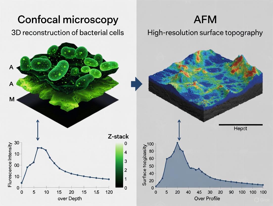
CLSM is an optical imaging technique that enables non-invasive optical sectioning of thick biological specimens, generating high-resolution 3D reconstructions of biofilm architecture without extensive physical sample preparation. The technique uses fluorescent staining to visualize specific biofilm components, including bacterial cells and EPS matrix elements, under physiological conditions.

Recent Experimental Application: A 2025 study successfully employed CLSM combined with scanning ion conductance microscopy (SICM) to visualize the 3D morphology of marine bacterial (Aliivibrio fischeri) biofilms on glass substrates in phosphate buffer solution [3]. Researchers fixed biofilms with glutaraldehyde and applied dual staining with crystal violet (targeting negatively charged cell membranes) and DAPI (staining bacterial DNA). The system generated 3D images from 166 optical sections taken at approximately 130nm intervals in the Z-direction, revealing both structural organization and bacterial arrangement within the biofilm [3].

Atomic Force Microscopy (AFM)

AFM utilizes a physical probe to scan surfaces at nanometer resolution, providing topographical imaging and quantitative mechanical property mapping under physiological conditions. Unlike CLSM, AFM requires no staining or extensive sample preparation and can simultaneously characterize structural and mechanical properties of biofilms.

Recent Experimental Application: A 2025 study introduced an automated large-area AFM approach capable of capturing high-resolution images over millimeter-scale areas, overcoming traditional AFM limitations of small imaging areas (<100µm) [4]. The system imaged Pantoea sp. YR343 biofilms on PFOTS-treated glass surfaces, revealing cellular orientation patterns and honeycomb structures during early biofilm formation. Machine learning algorithms assisted with image stitching, cell detection, and classification, enabling visualization of flagellar structures measuring 20-50nm in height and tens of micrometers in length [4]. In a separate 2025 mechanical properties study, AFM measured Young's modulus of Staphylococcus epidermidis biofilms following EPS modification treatments, demonstrating how specific matrix components influence biofilm mechanical strength [2].

Technical Comparison: CLSM vs. AFM

Table 1: Technical Specifications and Capabilities Comparison

Parameter	Confocal Laser Scanning Microscopy (CLSM)	Atomic Force Microscopy (AFM)
Resolution	~200-300nm lateral; ~500-700nm axial [3]	Nanometer scale (sub-cellular features ~20-50nm) [4]
Imaging Depth	Up to several hundred micrometers (limited by light penetration)	Surface topography and near-surface mechanical properties
Sample Requirements	Typically requires fluorescent staining/ labeling	No staining required; can image in liquid and air
Sample Preservation	Non-invasive; enables live cell imaging	Potential for sample deformation with soft EPS [3]
Key Measurables	3D architecture, cellular arrangement, component localization via staining	Topography, mechanical properties (Young's modulus, adhesion) [2]
Field of View	Millimeter-scale with appropriate objectives	Millimeter-scale with automated large-area systems [4]
Complementary Techniques	SICM for simultaneous topography and ion conductivity [3]	FTIR for chemical composition [2]
Data Output	3D fluorescence reconstruction	3D topographical maps, force spectroscopy data
Best Applications	Visualizing biofilm architecture, cell distribution, and viability assessment in hydrated samples	Nanoscale surface features, mechanical properties, and early attachment dynamics

Table 2: Experimental Data from Recent Studies (2025)

Study Focus	Technique	Key Quantitative Findings	Implications
EPS-Mechanical Properties Relationship [2]	AFM	Young's modulus significantly changed (p<0.05) with EPS composition; Proteinase K reduced biovolume by 65%	EPS composition directly governs biofilm mechanical stability
Early Biofilm Formation [4]	Large-area AFM	Cells: ~2µm length, ~1µm diameter; Flagella: 20-50nm height; Honeycomb patterns at 6-8h	Revealed nanoscale cellular orientation and appendage coordination in early attachment
Marine Biofilm Structure [3]	CLSM-SICM correlative	166 optical sections at 130nm intervals; Clear 3D reconstruction of hydrated architecture	Enabled simultaneous morphology visualization and bacterial arrangement mapping
3D Cancer Spheroid Mechanics [5]	AFM SmartMapping	Mechanical maps of entire spheroid surfaces (>150µm) revealing heterogeneity	Demonstrated capability for large-scale 3D mechanical characterization

Experimental Protocols

• Biofilm Growth: Culture biofilms on appropriate substrates (e.g., glass-bottom dishes) under controlled conditions for desired duration.
• Fixation: Treat samples with 4% glutaraldehyde in phosphate-buffered saline (PBS) for 1 hour to preserve structure.
• Staining: Apply sequential staining:
  • Crystal violet solution (1 hour) for negatively charged cell membranes
  • DAPI solution (5-10 minutes) for bacterial DNA
• Imaging: Use confocal microscope with appropriate laser wavelengths (405nm for DAPI, 561nm for crystal violet) and emission filters.
• 3D Reconstruction: Capture Z-stack images at precise intervals (e.g., 130nm) and reconstruct using specialized software.

• Biofilm Growth: Grow biofilms under controlled shear conditions using CDC biofilm reactor for 12 days.
• EPS Modification: Treat with specific modifying agents:
  • Enzymes: Proteinase K (proteins), DNase I (eDNA), Lipase (lipids)
  • Chemicals: Periodic acid (polysaccharides), Ca²⁺/Mg²⁺ (cross-linking)
• AFM Measurement:
  • Conduct force spectroscopy measurements in appropriate buffer
  • Use colloidal probes or sharp tips depending on resolution requirements
  • Map multiple locations for statistical significance
• Data Analysis: Calculate Young's modulus from force-distance curves using appropriate contact mechanics models (e.g., Hertz, Sneddon).

Visualizing the Workflows

Research Reagent Solutions

Table 3: Essential Research Reagents and Materials

Reagent/Material	Function	Application Examples
Crystal Violet	Stains negatively charged cell membranes and EPS components	CLSM visualization of biofilm structure [3]
DAPI (4′,6-Diamidino-2-phenylindole)	Fluorescent DNA binding dye for nuclear staining	Identifying bacterial cells within biofilm matrix [3]
Proteinase K	Protease enzyme that degrades protein components of EPS	Studying contribution of proteins to mechanical properties [2]
DNase I	Enzyme that cleaves extracellular DNA (eDNA) in EPS	Evaluating eDNA role in biofilm stability [2]
Periodic Acid	Chemical that oxidizes and cleaves polysaccharides	Assessing polysaccharide contribution to matrix integrity [2]
Glutaraldehyde	Cross-linking fixative for structural preservation	Sample preparation for microscopy [3]
PFOTS-treated Glass	Hydrophobic surface modification	Studying surface attachment dynamics [4]
Marine Broth 2216	Culture medium for marine bacteria	Growing Aliivibrio fischeri biofilms [3]

The future of biofilm architecture analysis lies in correlative approaches that combine multiple techniques. As noted in a 2025 market analysis, "Hybrid microscopy platforms provide multidimensional insights, making them ideal for advanced materials science and biological research" [6]. The integration of AI and machine learning is transforming both CLSM and AFM, enabling automated image analysis, enhanced resolution, and quantitative data extraction [4] [7]. For instance, AI-driven models now optimize AFM scanning processes and automate probe conditioning, while ML algorithms assist with seamless image stitching over millimeter-scale areas [4].

For researchers and drug development professionals, the choice between CLSM and AFM depends on specific research questions. CLSM excels at visualizing 3D architecture and spatial relationships in fully hydrated, living biofilms, making it ideal for studying biofilm development and response to antimicrobial treatments. AFM provides unparalleled nanoscale resolution of surface features and quantitative mechanical properties, crucial for understanding surface interactions and material impacts on biofilm formation. The most comprehensive understanding emerges when these techniques are used complementarily, leveraging their respective strengths to overcome their limitations.

As biofilm-related challenges continue to impact clinical outcomes and industrial processes, advanced architectural analysis using these sophisticated imaging platforms will be instrumental in developing targeted anti-biofilm strategies. The integration of these technologies with emerging approaches in nanotechnology, synthetic biology, and computational analysis promises to accelerate breakthroughs in biofilm management across diverse applications.

Core Principles of Confocal Microscopy

Confocal Laser Scanning Microscopy (CLSM) is a powerful optical imaging technique that revolutionized biological sciences by enabling high-resolution, three-dimensional imaging of thick specimens. The fundamental principle, patented by Marvin Minsky in 1957, involves the use of a spatial pinhole to block out-of-focus light during image formation [8] [9]. This core mechanism provides the two defining capabilities of CLSM: significantly improved optical resolution and optical sectioning for 3D reconstruction [9].

In a conventional wide-field fluorescence microscope, the entire specimen is evenly illuminated, and light from above and below the focal plane contributes to a blurred background haze in the final image [8]. In contrast, a confocal microscope illuminates a single, diffraction-limited spot at a time with a laser beam. The emitted fluorescent or reflected light from this spot is then focused through a second pinhole aperture situated in front of the detector. This "confocal" pinhole is positioned at a conjugate focal plane to the illuminated spot, ensuring that only the in-focus light passes through to the detector, while the out-of-focus light is physically blocked [8] [10]. This process is described by the point spread function (PSF), which models the diffraction pattern of a point source and is key to the enhanced resolution [10].

To build a complete two-dimensional image, this illumination spot is raster-scanned across the sample using precisely controlled oscillating mirrors [8] [11]. A complete 3D image, or z-stack, is then assembled by sequentially capturing images at different depth levels (focal planes) within the specimen [9]. These optical sections can be digitally processed to reconstruct a high-fidelity three-dimensional model of the sample without the need for physical sectioning [8] [11].

Visualizing the Confocal Principle

The following diagram illustrates the key components and light path of a Confocal Laser Scanning Microscope.

CLSM in Biofilm Architecture Analysis

CLSM is an indispensable tool in biofilm research, allowing scientists to study the complex three-dimensional architecture of these microbial communities in a non-invasive manner [12] [13]. Biofilms are surface-attached communities of microorganisms enclosed in a self-produced matrix of extracellular polymeric substances (EPS) [4]. Their 3D structure is critical to their function and resistance to antimicrobials.

A primary application of CLSM in this field is the quantitative evaluation of structural parameters such as biofilm biomass, thickness, roughness, and substratum coverage [12]. When used with viability stains or species-specific fluorescent probes (e.g., FISH), CLSM can spatially resolve the distribution of live/dead cells or identify different bacterial species within a multispecies biofilm, providing insights into interspecies interactions and the effects of antimicrobial treatments [12] [14].

Experimental Protocol for Biofilm Imaging with CLSM

A standard workflow for analyzing biofilm architecture using CLSM involves several key steps [12] [14]:

• Sample Preparation: Biofilms are grown on a suitable substrate (e.g., glass coverslips, relevant industrial surfaces). The biofilm is then stained with one or more fluorescent dyes. Common stains include:
  • SYTO 9: A green-fluorescent nucleic acid stain that labels all cells.
  • Propidium Iodide (PI): A red-fluorescent nucleic acid stain that penetrates only cells with damaged membranes, thus labeling dead cells. Used in combination with SYTO 9 for viability assessment.
  • Concanavalin A or other lectins: Conjugated to a fluorophore (e.g., tetramethylrhodamine) to specifically label polysaccharide components of the EPS matrix.
• Image Acquisition: The stained biofilm is mounted on the microscope stage. Using a water- or oil-immersion objective with high numerical aperture (NA), a z-stack is acquired. The step size between optical sections (e.g., 0.5 - 1 µm) is set to adequately sample the biofilm thickness. The pinhole diameter is typically set to 1 Airy Unit to optimize sectioning thickness and signal-to-noise ratio [11].
• 3D Reconstruction and Analysis: The acquired z-stack of 2D images is processed using specialized software (e.g., ImageJ, IMARIS, COMSTAT). The software reconstructs a 3D volume from which quantitative parameters like biovolume (µm³/µm²), average thickness (µm), and surface roughness are extracted.

The Scientist's Toolkit: Essential Reagents for CLSM Biofilm Analysis

Research Reagent / Material	Function in CLSM Biofilm Analysis
Fluorescent Nucleic Acid Stains (e.g., SYTO 9, DAPI)	To label and visualize all bacterial cells within the biofilm community based on DNA/RNA content [12].
Viability Stains (e.g., Propidium Iodide)	To differentiate between live and dead cell populations when used in combination with other cell-permeant stains [12].
Fluorescently-Labelled Lectins (e.g., ConA-TRITC)	To bind to and visualize specific sugar residues in the exopolysaccharide (EPS) matrix, revealing its structure and composition [14].
High NA Objective Lens	To collect maximum light and achieve high resolution; water-immersion objectives are ideal for live hydrated biofilms [8].
Mounting Medium	To preserve the native 3D structure of the biofilm and, if using oil-immersion objectives, to match the refractive index for optimal image quality [8].

CLSM vs. Atomic Force Microscopy (AFM) for Biofilm Research

While CLSM excels at visualizing 3D internal architecture, Atomic Force Microscopy (AFM) provides complementary, high-resolution data on surface topography and nanomechanical properties. The choice between them depends heavily on the research question.

Direct Comparison of Techniques

The table below summarizes the core differences between CLSM and AFM in the context of biofilm analysis.

Parameter	Confocal Laser Scanning Microscopy (CLSM)	Atomic Force Microscopy (AFM)
Primary Data	3D fluorescence imaging, optical sections	3D surface topography, nanomechanical force maps
Resolution	~0.2 µm lateral, ~0.6 µm axial [8]	Nanometer-scale (sub-cellular, molecular) [4]
Sample Environment	Hydrated, live samples possible; can image through coverslips	Typically in liquid or air; probes the immediate surface
Key Applications in Biofilm Research	3D architecture, thickness, biovolume, cell viability, co-localization studies [12] [14]	Surface roughness, adhesion forces, elasticity, visualization of appendages like flagella [12] [4]
Sample Preparation	Often requires fluorescent staining	Minimal preparation; no staining required
Throughput	Relatively high; can image large areas quickly	Traditionally low; slow scanning of small areas (<100µm) [4]
Key Limitation	Limited by light diffraction; photobleaching of fluorophores [12]	Small scan area; potential for surface deformation; cannot image subsurface features [12] [4]

Synergistic Use: CLSM and AFM

The most powerful insights often come from using CLSM and AFM in tandem. CLSM can identify regions of interest based on 3D structure and cell viability, after which AFM can target those specific areas to measure mechanical properties or image surface features at the nanoscale [14]. For example, CLSM could reveal a heterogeneous biofilm with dense clusters of cells, and AFM could then be used to show that these clusters are significantly stiffer than the surrounding EPS-rich areas, a finding demonstrated in Pseudomonas biofilms [12].

Recent advancements, such as large-area automated AFM combined with machine learning for image stitching, are addressing the traditional throughput limitations of AFM. This new approach allows for high-resolution mapping over millimeter-scale areas, bridging the gap between nanoscale features and the functional macroscale organization of biofilms [4]. This evolution makes correlative CLSM-AFM studies even more feasible and powerful.

Confocal Laser Scanning Microscopy stands as a cornerstone technique for the analysis of biofilm architecture, providing unparalleled capabilities for non-invasive, three-dimensional imaging and quantification. Its strength lies in visualizing the internal structure and composition of hydrated, living biofilms across scales relevant to their function. While AFM provides superior resolution for surface topography and nanomechanical property mapping, the two techniques are highly complementary. The future of biofilm research lies in leveraging these multimodal approaches, combining the 3D structural context from CLSM with the nanoscale surface and mechanical data from advanced AFM to build a comprehensive understanding of biofilm assembly, resilience, and function.

Atomic Force Microscopy (AFM) is a very-high-resolution type of scanning probe microscopy (SPM) that provides resolution on the order of fractions of a nanometer, more than 1000 times better than the optical diffraction limit [15]. Unlike optical or electron microscopy, AFM does not use lenses or beam irradiation but operates by "feeling" or "touching" the surface with a sharp mechanical probe [15]. This fundamental difference allows AFM to overcome limitations of diffraction and aberration, enabling researchers to characterize surface topography and material properties at the atomic scale without extensive sample preparation or vacuum conditions [15].

The technique has evolved significantly since its invention by IBM scientists in 1986 [15], expanding from basic topographic imaging to a comprehensive toolkit for nanoscale mechanical, electrical, and chemical characterization. AFM's versatility makes it indispensable across numerous disciplines, including solid-state physics, polymer chemistry, molecular biology, and biomedical research [15]. In the specific context of biofilm architecture analysis, which is central to our comparative thesis, AFM provides unique capabilities for investigating the structural and mechanical properties of microbial communities under physiological conditions.

Fundamental Operating Principles of AFM

Core Components and Mechanism

The AFM instrument consists of several key components that work together to probe surface properties [16]:

• Cantilever: A small spring-like lever typically made of silicon or silicon nitride
• Sharp Tip: A probe with a tip radius of curvature on the order of nanometers, fixed to the free end of the cantilever
• Piezoelectric Scanner: Controls the precise movement of the tip or sample in x, y, and z directions with sub-nanometer accuracy
• Detection System: Most commonly uses a laser beam reflected from the back of the cantilever onto a position-sensitive photodetector
• Feedback Loop: Maintains constant interaction force between tip and sample during scanning

The underlying principle involves measuring the interaction forces between the sharp tip and the sample surface. As the tip approaches the surface, forces cause the cantilever to bend or deflect. This deflection is tracked by the laser and photodetector system, and the feedback loop adjusts the tip-sample separation to maintain a constant interaction force [17]. By raster scanning the tip across the sample surface and recording these adjustments, a three-dimensional topographic image is constructed [16].

Primary Imaging Modes

AFM operates in several distinct modes, each optimized for specific applications and sample types [16]:

• Contact Mode: The tip maintains constant contact with the sample surface during scanning. The feedback loop maintains constant cantilever deflection, corresponding to constant force. Soft cantilevers (≤1 N/m) are typically used to minimize tip wear and surface damage.

• Tapping Mode (Intermittent Contact): The cantilever is oscillated at or near its resonance frequency, and the tip makes intermittent contact with the surface. This reduces lateral forces and minimizes sample damage, making it suitable for soft samples.

• Non-Contact Mode: The cantilever oscillates near the surface without making contact, sensing attractive van der Waals forces. This mode offers the lowest interaction forces but can be challenging to implement.

Advanced Characterization Modes

Beyond topography, AFM enables numerous specialized characterization techniques through variations of the basic operating modes [16]:

• Phase Imaging: Records phase differences between drive signal and cantilever oscillation to map material properties like elasticity and adhesion
• Force Modulation: Maps elastic properties by analyzing cantilever response to periodic vertical modulation
• Lateral Force Microscopy (LFM): Detects torsional twisting of the cantilever to measure friction forces
• Force-Distance Measurements: Quantifies mechanical properties, adhesion, and molecular interactions through approach-retract curves
• Magnetic Force Microscopy (MFM): Images magnetic field distributions using magnetically-coated tips
• Electrical Modes: Including Scanning Spreading Resistance Microscopy (SSRM) and Kelvin Probe Force Microscopy (KPFM) for mapping electrical properties
• Nanomechanical Mapping: Advanced techniques like force volume mode that generate spatial maps of mechanical properties

AFM Applications in Biofilm Research

High-Resolution Structural Analysis

AFM enables detailed structural characterization of biofilms at the nanoscale, revealing features inaccessible to optical techniques. Recent studies demonstrate AFM's capability to visualize not only bacterial cells but also fine extracellular structures. For instance, research on Pantoea sp. YR343 biofilms revealed flagellar structures measuring approximately 20-50 nm in height and extending tens of micrometers across surfaces [4]. These appendages, critical for surface attachment and biofilm assembly, would be challenging to resolve with conventional microscopy.

The technique particularly excels at visualizing the extracellular polymeric substance (EPS) matrix that constitutes the biofilm scaffold. AFM can resolve the three-dimensional architecture of this matrix under physiological conditions, providing insights into how polysaccharides, proteins, extracellular DNA, and lipids organize to form the biofilm infrastructure [18]. This structural information is crucial for understanding biofilm stability, nutrient transport, and resistance mechanisms.

Nanomechanical Property Mapping

AFM-based mechanical property measurements have become essential tools for quantifying biofilm mechanical behaviors [19]. By using force-distance curves and contact mechanics models, researchers can generate spatial maps of properties including:

• Young's modulus (stiffness/elasticity)
• Adhesion forces
• Viscoelastic properties
• Deformation characteristics

These measurements reveal how mechanical properties vary spatially within biofilms, correlating structural features with functional behaviors. For example, studies have demonstrated that different EPS components contribute distinctly to biofilm mechanical integrity. Protein-dominated EPS matrices exhibit different mechanical signatures compared to polysaccharide-rich regions [2].

Advanced nanomechanical mapping techniques like force volume, nano-DMA, and parametric modes enable comprehensive mechanical characterization [19]. Force volume involves acquiring force-distance curves at each pixel of the sample surface, while nano-DMA applies oscillatory signals to measure viscoelastic properties. Parametric methods derive mechanical properties from cantilever oscillation parameters without explicitly acquiring force-distance curves.

Investigating EPS-Dependent Mechanical Properties

The relationship between EPS composition and biofilm mechanical properties represents a key application of AFM in biofilm research. A fundamental study treating Staphylococcus epidermidis biofilms with EPS-modifying agents demonstrated AFM's sensitivity to compositional changes [2]. The experimental protocol involved:

• Growing pure culture biofilms in CDC biofilm reactors under controlled conditions
• Applying targeted EPS modifiers including proteases, lipases, nucleases, and periodic acid
• Using AFM to measure Young's modulus changes following treatments
• Correlating mechanical properties with compositional analysis (FTIR) and structural characterization (CLSM)

Results demonstrated that enzymatic degradation of specific EPS components significantly altered biofilm mechanical properties, with protease treatment causing the most substantial reduction in mechanical strength [2]. This approach provides insights for developing EPS-targeted biofilm control strategies.

Table 1: Research Reagent Solutions for AFM Biofilm Mechanical Analysis

Reagent/Agent	Target EPS Component	Mechanical Effect	Experimental Function
Protease K	Proteins	Significant reduction in Young's modulus	Degrades peptide bonds in extracellular proteins
Periodic Acid	Polysaccharides	Alters viscoelastic properties	Oxidizes vicinal hydroxyl groups in carbohydrates
DNase I	Extracellular DNA (eDNA)	Reduces cohesion	Cleaves DNA backbone in extracellular matrix
Lipase	Lipids	Minor mechanical changes	Hydrolyzes ester bonds in extracellular lipids
Ca²⁺ ions	Cross-linking	Increases stiffness	Enhances ionic bridging between polymer chains

Comparative Analysis: AFM vs. Confocal Microscopy for Biofilm Architecture

Technical Capabilities and Limitations

When selecting techniques for biofilm architecture analysis, researchers must consider the complementary strengths and limitations of AFM and confocal microscopy:

Table 2: AFM vs. Confocal Microscopy for Biofilm Research

Parameter	Atomic Force Microscopy (AFM)	Confocal Laser Scanning Microscopy
Maximum Resolution	Sub-nanometer (atomic scale possible) [15]	~200 nm (diffraction-limited) [17]
Imaging Environment	Air, liquids, vacuum [16]	Typically aqueous or fixed samples
Sample Preparation	Minimal; no staining required [14]	Often requires fluorescent labeling
Depth Penetration	Surface and near-surface (μm range)	50-100 μm in transparent samples [14]
Measurement Type	Topography, mechanical, electrical properties [16]	Optical sections, chemical specificity
Throughput	Slow to moderate (minutes to hours)	Relatively fast (seconds to minutes)
Live Cell Imaging	Possible under physiological conditions [4]	Excellent with viability-compatible dyes
Quantitative Data	Nanomechanical properties, adhesion forces [19]	Concentration, thickness, viability

Operational Workflows and Data Output

The fundamental differences between AFM and confocal microscopy extend beyond specifications to encompass distinct operational paradigms and data outputs:

Integrated Approaches for Comprehensive Biofilm Characterization

Rather than positioning AFM and confocal microscopy as competing techniques, advanced biofilm research increasingly employs integrated approaches that leverage their complementary strengths:

• Correlative Microscopy: Combining AFM nanomechanical data with confocal 3D structural information from the same sample region
• Structural-Functional Relationships: Relating AFM-measured mechanical properties to composition data from fluorescence labeling
• Multi-scale Analysis: Using confocal microscopy to identify regions of interest for high-resolution AFM interrogation
• Dynamic Studies: Monitoring biofilm development over time with confocal imaging, with periodic AFM characterization of mechanical evolution

This integrated methodology provides a more comprehensive understanding of biofilm architecture, bridging the gap between nanoscale material properties and microscale community organization.

Experimental Protocols for AFM Biofilm Analysis

Sample Preparation Methodologies

Proper sample preparation is critical for successful AFM analysis of biofilms. Common approaches include:

• Substrate Selection: Biofilms are typically grown on flat substrates compatible with AFM scanning, such as glass coverslips, silicon wafers, or mica sheets. Surface treatment (e.g., PFOTS-silanization) may be used to promote adhesion [4].

• In Situ Growth: Biofilms are grown directly on AFM-compatible substrates under controlled conditions. For flow-based systems, biofilms can be grown in CDC biofilm reactors or flow cells, then transferred to the AFM [2].

• Hydration Maintenance: For biological AFM in liquid, samples must remain hydrated throughout transfer and measurement. Various liquid cells and chambers maintain physiological conditions during scanning.

• Minimal Processing: Unlike electron microscopy, AFM requires no fixation, dehydration, or metal coating, preserving native biofilm structure [14].

Nanomechanical Mapping Protocol

A typical protocol for nanomechanical mapping of biofilms includes these key steps [19] [2]:

• Cantilever Selection: Choose appropriate cantilevers based on sample stiffness and measurement mode. Soft cantilevers (0.1-1 N/m) are typically used for biological samples.

• Calibration: Determine cantilever spring constant using thermal tuning or reference measurements.

• Approach: Engage the tip with the surface using minimal force to avoid sample damage.

• Topography Imaging: Acquire baseline topographic data in tapping or contact mode.

• Force Mapping: Acquire force-distance curves at predetermined spatial intervals (e.g., 64×64 or 128×128 points).

• Data Analysis: Fit approach curves with appropriate contact mechanics models (Hertz, Sneddon, JKR) to extract mechanical parameters.

• Spatial Mapping: Generate mechanical property maps by assigning calculated parameters to corresponding spatial coordinates.

Advanced Mechanical Characterization

For comprehensive viscoelastic characterization, more advanced protocols may be employed:

• Nano-DMA: After establishing contact at a setpoint force, apply oscillatory signals at varying frequencies while monitoring cantilever response to characterize viscoelastic behavior [19].

• Force Volume: Acquire complete force-distance curves at each pixel, capturing both approach and retraction cycles to map adhesion and deformation properties simultaneously.

• Long-term Studies: Monitor mechanical property evolution during biofilm development or in response to chemical treatments using time-lapse nanomechanical mapping.

Future Directions and Methodological Advances

The field of AFM continues to evolve with technological improvements enhancing capabilities for biofilm research:

• High-Speed AFM: Increases imaging rates from minutes to seconds, enabling observation of dynamic processes [19] [16].

• Combined Microscopy Systems: Integrated AFM-confocal instruments facilitate direct correlation of structural and mechanical data.

• Machine Learning Integration: AI-assisted data analysis improves quantitative accuracy and enables automated feature recognition in complex biofilm structures [4].

• Advanced Probes: Specialized tips with functionalized coatings enable chemical force microscopy and specific molecular recognition.

• Environmental Control: Advanced fluid cells allow precise control of temperature, chemistry, and flow conditions during measurements.

These developments continue to expand AFM's utility in biofilm research, providing increasingly sophisticated tools to understand the complex structure-function relationships that govern biofilm behavior in medical, industrial, and environmental contexts.

Biofilms are structured microbial communities embedded in a self-produced extracellular polymeric substance (EPS) matrix, which determines the immediate conditions of life for biofilm cells by affecting porosity, density, water content, charge, and mechanical stability [20]. This complex, dynamic matrix is far more than simple "slime"; it is a highly functional scaffold, often termed the "matrixome," composed of a diverse array of biomolecules including polysaccharides, proteins, extracellular DNA (eDNA), lipids, and glycolipids [20] [21]. The spatial organization of microbial cells within this EPS matrix is critical to biofilm function, resilience, and virulence. Understanding this architecture requires advanced imaging techniques, primarily Confocal Laser Scanning Microscopy (CLSM) and Atomic Force Microscopy (AFM), which offer complementary insights into the biofilm's hidden world. This guide provides an objective comparison of these core technologies, supported by experimental data and detailed protocols, to inform their application in biofilm research and therapeutic development.

Table 1: Core Technique Comparison: CLSM vs. AFM

Feature	Confocal Laser Scanning Microscopy (CLSM)	Atomic Force Microscopy (AFM)
Primary Imaging Mode	Optical, fluorescence-based	Physical, probe-based
Key Measurable Parameters	3D architecture, cell location via staining, chemical composition, live-cell dynamics [22] [3]	Topography, nanomechanical properties (stiffness, adhesion), molecular interactions [4]
Resolution	Diffraction-limited (~200 nm laterally) [23]	Nanoscale (<100 nm, sub-nanometer vertically) [4]
In situ / Live Cell Capability	Excellent for real-time observation under physiological conditions [23]	Good; can be performed in liquid, but scan speed can limit dynamic studies [4]
Sample Preparation	Often requires staining or fluorescent tagging; can be minimal for live imaging [22]	Minimal; no staining or metal coatings required [4]
Key Advantage	Non-destructive 3D visualization of internal structure and composition in real time.	Unmatched resolution of surface topology and quantitative nanomechanical mapping.
Main Limitation	Resolution limit obscures nanoscale features; requires fluorescent labels.	Small scan area, potential for soft sample deformation, slower for large areas [4] [3].

Key Research Reagent Solutions

The following reagents and materials are essential for preparing and analyzing biofilm architecture using the discussed methodologies.

Table 2: Essential Research Reagents and Materials

Item	Function/Application	Example Use in Protocols
Fluorescent Stains (e.g., DAPI, Calcofluor White, Congo Red)	Label specific biofilm components (e.g., DNA, polysaccharides) for CLSM visualization [3] [24].	Differentiating bacterial cells from EPS in the dual-staining method [24].
Maneval's Stain	A simple, cost-effective dye for visualizing and differentiating bacterial cells (magenta-red) from the polysaccharide matrix (blue) under light microscopy [24].	Used in the novel dual-staining method for basic biofilm differentiation [24].
Glutaraldehyde & Formaldehyde	Fixatives used to preserve biofilm structure for analysis by techniques like SEM and CLSM [3] [24].	Cross-linking and preserving biofilm structure prior to SEM imaging [24].
Polydimethylsiloxane (PDMS) Flow Cells	Microfluidic devices that facilitate real-time, in situ growth and observation of biofilms under controlled shear stress [23].	Monitoring dynamic biofilm formation and development in real time [23].
Metal-Organic Frameworks (MOFs)	Nanostructured coatings that act as mechano-bactericidal surfaces, physically puncturing bacteria to limit biofilm formation [25].	Coating surfaces to study and prevent initial bacterial attachment [25].

Experimental Protocols for Biofilm Visualization

CLSM for 3D Architecture and Composition

Application: This protocol is ideal for visualizing the three-dimensional structure of a biofilm, locating different microbial species, and mapping the distribution of EPS components in a hydrated, near-native state [22] [3].

Detailed Methodology:

• Biofilm Growth: Grow biofilms on suitable substrates (e.g., glass-bottom dishes) under desired conditions. For dynamic studies, use flow cells to control nutrient supply and shear force [23].
• Staining: Apply fluorescent probes to the biofilm.
  • For total biomass or EPS: Use stains like Crystal Violet (CV) [3].
  • For nucleic acids (labeling cells): Use DAPI [3].
  • For specific microbial taxa: Use Fluorescence In Situ Hybridization (FISH) with targeted oligonucleotide probes [22].
• Fixation (Optional): For endpoint analysis, fix biofilms with a solution like 4% glutaraldehyde in phosphate-buffered saline (PBS) for 1 hour to preserve structure [3].
• Imaging: Use a confocal microscope to capture Z-stacks (optical sections) through the biofilm depth. The resulting stack is reconstructed into a 3D model for analysis of biovolume, thickness, and spatial co-localization [22] [26].

Large-Area Automated AFM for Nanoscale Topography

Application: This advanced AFM protocol is used to achieve high-resolution, nanoscale images of biofilm surface topography, cellular morphology, and appendages (e.g., flagella) over millimeter-scale areas, overcoming traditional AFM's limited scan range [4].

Detailed Methodology:

• Sample Preparation: Grow biofilms on a flat, solid substrate (e.g., PFOTS-treated glass). Gently rinse to remove unattached cells and air-dry [4]. Note that drying may alter native structure, though liquid imaging is possible.
• Automated Scanning: Implement an automated large-area AFM system. The system collects multiple contiguous high-resolution images (e.g., 100x100 µm) across the biofilm surface.
• Image Stitching and Analysis: Use machine learning (ML) algorithms to seamlessly stitch the individual images into a single, large millimeter-scale topographic map. Subsequent ML-driven analysis can automatically detect cells, classify features, and quantify parameters like cell count, orientation, and confluency [4].

Correlative SICM-CLSM for In-situ Nanostructure

Application: This correlative protocol provides a comprehensive view by combining the nanoscale surface morphology from Scanning Ion Conductance Microscopy (SICM) with the internal structural information from CLSM on the exact same sample area [3].

Detailed Methodology:

• Biofilm Generation: Grow biofilms on a transparent, conductive substrate like a gridded glass slide.
• Fixation and Staining: Fix the biofilm with glutaraldehyde and stain with fluorescent dyes (e.g., DAPI for DNA, CV for membranes) as in the CLSM protocol [3].
• Correlative Imaging:
  • First, use CLSM to obtain a 3D fluorescence image, identifying locations of bacterial cells and matrix components.
  • Then, use SICM to scan the identical region. SICM uses a nanopipette in a liquid environment to map the 3D surface topography without physical contact, preventing deformation of soft EPS [3].
• Data Integration: Overlay the CLSM and SICM datasets to correlate the internal cellular arrangement with the nanoscale surface features and local ion conductivity, providing a multi-parameter view of the biofilm's structure [3].

Workflow for CLSM Analysis

Workflow for Automated AFM Analysis

Comparative Analysis and Emerging Trends

The choice between CLSM and AFM is not a matter of superiority but of application. CLSM excels at revealing the internal "blueprint" of the biofilm in 3D, while AFM provides an "as-built" survey of its nanoscale landscape and material properties. The emerging trend is to move beyond these techniques in isolation. Correlative microscopy, such as SICM-CLSM, combines their strengths to link nanoscale surface features with internal biochemical composition [3].

Furthermore, the integration of artificial intelligence (AI) and machine learning (ML) is transforming both techniques. In AFM, ML enables automated image stitching, cell classification, and distortion correction, making large-area nanoscale analysis feasible [4]. In CLSM and other omics-techniques, AI algorithms can process vast datasets of time-series images to identify patterns in population growth and spatial organization that are imperceptible to the human eye [27] [23]. One study of Streptococcus mutans biofilms used such computational analysis to reveal that biofilm assembly follows a power law and exhibits spatial-structural features resembling urbanization, where only a subset of "active colonizers" grow into microcolonies that merge into larger superstructures [26].

The future of biofilm visualization lies in hybrid approaches. Combining the high-resolution structural and mechanical data from AFM with the compositional and dynamic imaging capabilities of CLSM—and supplementing them with spectroscopic data and AI-powered analysis—will provide the holistic, multi-scale understanding needed to develop robust strategies to control detrimental biofilms and harness beneficial ones.

Methodological Deep Dive: Practical Applications of CLSM and AFM in Biofilm Research

In the study of complex microbial communities, understanding biofilm architecture is paramount, as its three-dimensional structure directly influences bacterial resilience, pathogenicity, and ecological function. Two powerful techniques dominate this architectural analysis: Confocal Laser Scanning Microscopy (CLSM) and Atomic Force Microscopy (AFM). This guide provides an objective comparison of their performance, underpinned by experimental data, to aid researchers in selecting the appropriate tool for their specific investigative needs.

CLSM utilizes laser light to capture high-resolution optical images at various depths within a sample, enabling non-invasive, three-dimensional, and real-time (4D) visualization of living biofilms, often through the use of fluorescent labeling [12] [28]. In contrast, AFM employs a physical probe to scan surfaces, providing exceptional topographical detail and nanomechanical properties at the sub-cellular level, typically without the need for extensive sample preparation or labeling [4] [14]. The choice between these methods hinges on the research question—whether it demands the observation of dynamic processes in live cells or the quantification of ultrastructural and physical properties at the nanoscale.

Performance Comparison: CLSM and AFM at a Glance

The following table summarizes the core capabilities, advantages, and limitations of CLSM and AFM, providing a clear, data-driven foundation for their comparison.

Table 1: Key Performance Characteristics of CLSM and AFM in Biofilm Research

Feature	Confocal Laser Scanning Microscopy (CLSM)	Atomic Force Microscopy (AFM)
Maximum Resolution	~200-250 nm (lateral) [12]	Nanometer scale (sub-cellular) [4]
Working Environment	Physiological conditions (liquid, live cell imaging) [29] [28]	Ambient air, liquids, or vacuum [4] [14]
Dimensional Imaging	3D + time (4D) [29] [12]	3D surface topography [4]
Key Applications	- Live-cell dynamics & viability [12] [28]- 4D spatial architecture [29]- Multi-species localization [28]	- Nanoscale topography & roughness [4] [14]- Nanomechanical properties [4]- Visualization of appendages (e.g., flagella) [4]
Sample Preparation	Often requires fluorescent staining, which may alter biofilm properties [12] [28]	Minimal preparation; no staining required, but drying may be needed [4] [14]
Primary Limitations	- Limited by laser penetration [14]- Potential phototoxicity to live cells [30]- Resolution barrier for fine structures	- Small scan area (<100 µm) [4]- Slow scanning speed [4]- Potential surface damage from tip [12]

Experimental Protocols for Biofilm Analysis

CLSM Protocol for 4D Live-Cell Imaging of 3D Tissue Cultures

This protocol, adapted from a study on a 3D lung model, details the procedure for tracking cellular and particle dynamics over 24 hours [29].

• Sample Holder Preparation: A custom 3D-printed sample holder with a twist-fastener lock mechanism is used to hang permeable membrane inserts in a glass-bottom dish. This maintains a minimal distance (<0.5 mm) between the insert membrane and the glass, compatible with long-working-distance objectives [29].
• Cell Labeling: Different cell types within the 3D co-culture are labeled with distinct, live-cell compatible fluorophores (e.g., Vybrant DiD). For particle uptake studies, fluorescently-labeled particles such as rhodamine B-labeled silica are used [29].
• Microscopy Acquisition: Imaging is performed on a confocal laser scanning microscope with a 20x magnification lens. Data is acquired in z-stack mode (e.g., 2 µm slice thickness) and time-lapse mode (e.g., 15-20 minute intervals) to create a 4D dataset. Sequential scanning of emission channels prevents signal overlap [29].
• Data Processing: The raw z-stack data is processed and rendered using 3D rendering software to visualize cell tracks, interactions, and particle uptake kinetics. Parameters like cell motility speed (µm/min) can be quantified from the tracks [29].

CLSM Protocol for Biofilm Architecture Under Simulated Microgravity

This protocol enables the study of biofilm formation under simulated microgravity with minimal architectural disruption [28].

• Bacterial Strain Preparation: Fluorescent protein-expressing bacterial strains (e.g., S. mutans constitutively expressing GFP, S. gordonii constitutively expressing DsRed) are grown to the desired phase [28].
• Biofilm Growth on RPM: The bacterial culture is diluted in a biofilm-promoting medium and inoculated into a glass-bottomed 96-well plate. The plate is then placed on a Random Positioning Machine (RPM), which is set to simulated microgravity (0 × g). Control plates are maintained statically at 1 × g [28].
• Direct Imaging: After incubation (e.g., 24 hours), the biofilms are imaged directly without washing or harvesting. Using an inverted confocal microscope, 3D z-stack images are acquired at high magnification (e.g., 400x) [28].
• Quantification: The z-stack images are analyzed to determine biovolume (µm³) and assess qualitative structural changes, such as the formation of tower-like structures or changes in density [28].

AFM Protocol for High-Resolution Analysis of Biofilm Assembly

This protocol leverages automated large-area AFM to link nanoscale features to millimeter-scale biofilm organization [4].

• Surface Preparation & Inoculation: A substrate (e.g., PFOTS-treated glass coverslip) is placed in a petri dish and inoculated with the bacterial strain of interest (e.g., Pantoea sp. YR343) in a liquid growth medium [4].
• Sample Harvesting: At designated time points, the substrate is gently rinsed to remove non-attached cells and dried prior to imaging [4].
• Automated Large-Area AFM: The substrate is imaged using an AFM system equipped with automated stage control. Multiple high-resolution images are taken over millimeter-scale areas [4].
• Data Stitching and Analysis: Machine learning algorithms stitch the individual scans into a seamless, large-area image. Subsequent ML-based segmentation is used for automated cell detection, classification, and extraction of parameters like cell count, confluency, shape, and orientation [4].

The Scientist's Toolkit: Essential Research Reagents and Materials

Table 2: Key Reagents and Materials for CLSM and AFM Biofilm Studies

Item	Function/Application	Specific Examples
Glass-Bottom Culture Dishes	Provides an optically clear window for high-resolution imaging on inverted microscopes.	Used in 4D live-cell imaging of 3D cultures [29].
Permeable Membrane Inserts	Supports the growth of complex, multi-layered cell cultures that mimic physiological tissue barriers.	Essential for 3D lung model in co-culture studies [29].
Live-Cell Fluorescent Trackers	Labels specific cell types or organelles for tracking and identification in live samples over time.	Vybrant DiD for labeling immune cells; CellTracker dyes [29].
"Gentle" Rhodamine Probes	A new class of fluorophores with reduced phototoxicity, enabling longer time-lapse imaging.	GR555-mito for mitochondria; GR555-PM for plasma membrane [30].
Fluorescent Proteins	Enables constitutive or in-situ expression of fluorescent markers in bacterial cells.	sGFP and DsRed for labeling S. mutans and S. gordonii [28].
Functionalized Substrates	Surfaces with specific chemical treatments to study the impact of surface properties on bacterial adhesion.	PFOTS-treated glass to control hydrophobicity and adhesion [4].

Workflow and Pathway Visualization

The following diagram illustrates the key decision pathways and experimental workflows for selecting and applying CLSM and AFM in biofilm research.

CLSM and AFM are not mutually exclusive but rather complementary techniques. CLSM is unparalleled for the in-situ, volumetric, and temporal analysis of living biofilms, providing critical data on architecture and cell behavior under physiological conditions. AFM offers a unmatched resolution for surface topology and physical properties, revealing details of initial cell attachment, extracellular matrix components, and nanomechanical forces. The emerging trend of combining these modalities, along with the integration of machine learning for data analysis [4], is paving the way for a more holistic and quantitative understanding of biofilm dynamics, from the macro- to the nanoscale.

Biofilms are complex microbial communities that pose significant challenges in medical, industrial, and environmental contexts. Understanding their assembly, structure, and response to environmental stresses is crucial for developing effective control strategies. In this landscape, Atomic Force Microscopy (AFM) and Laser Scanning Confocal Microscopy (LSCM) have emerged as powerful, yet fundamentally different, techniques for biofilm analysis. While LSCM offers a window into the interior of living cells by imaging fluorescently tagged macromolecules, AFM provides nanometer-scale resolution of surface architecture and biomechanical properties under physiologically relevant conditions. This guide provides an objective comparison of these technologies, presenting experimental data and methodologies that highlight their complementary strengths in biofilm architecture analysis.

AFM operates by sensing the forces between a sharp probe and the sample surface, generating three-dimensional topographical images while simultaneously quantifying mechanical properties. Unlike electron microscopy techniques that require extensive sample preparation including dehydration, staining, or metal coating, AFM can image living microbial cells in buffer solution without such manipulations. LSCM, while superior for dynamic imaging of intracellular processes and three-dimensional reconstruction of biofilm structures, is limited by diffraction to resolutions typically >200 nm and requires fluorescent labeling that may alter biological activity.

Table 1: Fundamental Technique Comparison

Characteristic	Atomic Force Microscopy (AFM)	Laser Scanning Confocal Microscopy (LSCM)
Resolution	Nanoscale (sub-nm to nm) [31]	Diffraction-limited (typically >200 nm)
Sample Environment	Native conditions (air, liquid) [32] [31]	Typically requires controlled media
Sample Preparation	Minimal (no labeling required) [32]	Requires fluorescent labeling
Information Type	Surface topography, mechanical properties, adhesion [33] [19]	Internal structure, molecular localization, viability
Imaging Depth	Surface and near-surface (nm-µm)	Tens to hundreds of micrometers
Live Cell Imaging	Yes, under physiological conditions [33] [31]	Yes, but potential phototoxicity

Technical Comparison: Resolution, Capabilities, and Throughput

AFM Operating Modes for Biofilm Research

AFM offers multiple imaging modes optimized for different sample types and information needs. Tapping mode (also called intermittent contact or AC mode) operates by oscillating the cantilever at its resonant frequency while scanning the surface, minimizing lateral forces and making it ideal for soft, biological samples like biofilms. Contact mode maintains constant tip-sample contact with user-determined force, enabling faster scanning of stiffer surfaces but potentially damaging delicate biological structures. Force volume mode captures force-distance curves at each pixel, generating nanomechanical property maps including elasticity, adhesion, and deformation.

Recent advancements include quantitative imaging (QI) mode, which collects force-distance curves at every pixel in a high-resolution image without the lateral forces that can displace loosely attached samples. This multiparametric mode simultaneously produces data on height, surface stiffness, and adhesion at high resolution, making it particularly valuable for imaging challenging biological samples such as bacteria [33]. For viscoelastic characterization, nano-DMA (nano-scale Dynamic Mechanical Analysis) applies oscillatory signals to the tip while in contact with the sample, measuring the time lag between indentation and applied force to quantify energy dissipation and storage moduli [19].

Comparative Performance Metrics

Table 2: Performance Metrics for Biofilm Imaging

Parameter	AFM	LSCM
Spatial Resolution	Sub-nanometer vertical; nanometer lateral [31]	~200 nm lateral; ~500 nm axial
Temporal Resolution	Seconds to minutes per image (limitation for dynamics)	Milliseconds to seconds per frame
Field of View	Typically <100 µm [4]	Up to millimeters
Mechanical Property Mapping	Yes (elasticity, adhesion, viscoelasticity) [33] [19] [34]	No
Molecular Specificity	Limited (requires functionalized tips)	High (with fluorescent probes)
Structural Information	Surface ultrastructure, nanoscale features [4] [31]	3D internal architecture, cellular distribution

Experimental Approaches and Workflows

Correlative AFM-LSCM Imaging Protocol

Integrated AFM-LSCM produces complementary information on different cellular characteristics for a comprehensive picture of cellular behaviour. The following workflow describes the simultaneous real-time imaging of living cells in situ, producing multiplexed data on cell morphology and mechanics, surface adhesion and ultrastructure, and real-time localization of multiple fluorescently tagged macromolecules [33].

Large-Area AFM for Biofilm Assembly Analysis

Conventional AFM imaging is limited by small scan areas (<100 µm), restricting the ability to link nanoscale features to functional macroscale organization. Large-area automated AFM addresses this limitation by capturing high-resolution images over millimeter-scale areas, aided by machine learning for seamless image stitching, cell detection, and classification [4].

Protocol for Large-Area AFM Biofilm Imaging:

• Surface Preparation: Treat glass coverslips with PFOTS or other relevant surface treatments to control bacterial adhesion
• Biofilm Growth: Inoculate surfaces with bacterial cells (e.g., Pantoea sp. YR343) in appropriate growth medium and incubate for selected time periods (30 minutes to several hours)
• Sample Processing: Gently rinse coverslips to remove unattached cells and dry before imaging
• Automated AFM Imaging: Program the AFM to acquire multiple adjacent high-resolution images across millimeter-scale areas with minimal overlap (5-10%)
• Image Stitching: Apply machine learning algorithms to seamlessly merge individual images into a continuous large-area map
• Morphological Analysis: Use automated cell detection and classification to extract parameters including cell count, confluency, cell shape, and orientation

This approach has revealed previously obscured spatial heterogeneity and cellular morphology during early stages of biofilm formation, including preferred cellular orientation and distinctive honeycomb patterns in Pantoea sp. YR343 biofilms [4].

Key Research Reagents and Materials

Table 3: Essential Research Reagents and Solutions

Reagent/Solution	Function/Application	Example Use Case
Cell-Tak	Cell immobilization on substrates	Anchoring bacterial cells for AFM imaging during division [33]
Fluorescent Dyes (CellROX, SYTO 82)	Visualization of oxidative stress, nucleic acids	Monitoring ROS generation and cell viability during stressor exposure [33]
PFOTS-treated Glass	Hydrophobic surface for controlled cell adhesion	Studying initial attachment dynamics in biofilm formation [4]
Functionalized AFM Tips	Specific molecular interactions	Mapping peptidoglycan with vancomycin tips or polysaccharides with lectin tips [31]
2,4-Dichlorophenoxyacetic Acid	Model chemical stressor	Investigating cellular response to anthropogenic contaminants [33]

Data Outputs and Comparative Analysis

Quantitative Nanomechanical Properties Across Cell Types

AFM enables the quantification of mechanical properties that serve as sensitive indicators of cellular function and response to environmental stressors. The following data from a correlative AFM-QI-LSCM study illustrates how these properties vary across cell types and in response to chemical exposure.

Table 4: Nanomechanical Properties of Microbial and Human Cells

Cell Type	Condition	Young's Modulus	Adhesion Force	Surface Roughness	Key Findings
E. coli	Normal division	200-1500 kPa [33]	Varies with media	-	Stiffer at cell center (1-1.5 MPa) vs. edges (200-300 kPa)
E. coli	1 mM 2,4-D exposure	Altered elasticity	Changed adhesion	-	Loss of FtsZ-GFP Z-ring, increased ROS [33]
C. albicans	8 mM 2,4-D exposure	2-fold increase	2-fold increase	Significant reduction	Increased ROS but no change in tubulin2 or histone distribution [33]
HEK 293	Normal	-	Low adhesion	Smooth surface	Distinct tubulin network, low ROS signal [33]
HEK 293	1 mM 2,4-D, 30 min	Decreased	Significant increase	Decreased	Complete tubulin network disruption, cell shrinkage, rounding [33]

Integrated Data Interpretation

The correlation of AFM and LSCM data provides unprecedented insight into the relationship between structural/mechanical properties and intracellular processes. For example, in HEK 293 cells exposed to the herbicide 2,4-D, AFM detected a significant increase in adhesion and decrease in Young's modulus, while LSCM revealed disruption of the tubulin network and increased mitochondrial ROS that subsequently intensified in the nucleus [33]. This multiparametric assessment demonstrates how chemical stressors simultaneously alter physical cell properties and internal molecular arrangements.

Application in Antimicrobial Resistance and Biofilm Control

AFM has provided critical insights into antimicrobial resistance mechanisms, which is particularly relevant for biofilm-associated infections that demonstrate remarkable resilience against conventional treatments. Biofilms exhibit up to 1000-fold higher resistance to antimicrobial agents compared to planktonic bacteria, attributed to EPS-mediated diffusion barriers, metabolic dormancy, persister cells, and enhanced efflux-pump expression [1].

AFM investigations have revealed how bacteria adapt to antibiotics at the nanoscale, addressing the growing challenge of antimicrobial resistance. Studies comparing the mechanical properties of antibiotic-sensitive and resistant strains have identified correlations between cell wall stiffness and resistance mechanisms. For instance, AFM has been used to investigate changes in bacterial cell surface ultrastructure and mechanical properties following antibiotic exposure, providing insights into how structural adaptations contribute to resistance development [34].

In drinking water distribution systems, AFM has enabled in situ characterization of biofilm structural changes during free chlorine and monochloramine exposure. AFM images revealed a densely packed and heterogeneous biofilm structure before treatment, with substantial structural impact and detachment observed upon free chlorine exposure [35]. This application demonstrates how AFM can provide utilities with nanoscale insights to optimize disinfection strategies for biofilm control.

The study of biofilms, complex microbial communities encased in an extracellular polymeric substance (EPS), has been revolutionized by advanced microscopy techniques. Within the broader context of confocal laser scanning microscopy (CLSM) versus atomic force microscopy (AFM) for architectural analysis, this guide focuses on the unique capabilities of fluorescence-based CLSM methods. While AFM excels at providing high-resolution nanoscale topographical images and quantitative maps of nanomechanical properties under physiological conditions [4], CLSM techniques offer unparalleled insights into dynamic processes and chemical environments within living, hydrated biofilms without requiring extensive sample preparation that may introduce artifacts [12] [36].

Fluorescence Recovery After Photobleaching (FRAP) and Fluorescence Lifetime Imaging Microscopy (FLIM) represent two powerful approaches in the CLSM arsenal. FRAP investigates the mobility and diffusion coefficients of fluorescent molecules within the biofilm matrix, providing critical data on mass transport limitations that contribute to antimicrobial resistance [37]. FLIM, meanwhile, probes the local microenvironment of fluorophores, with lifetime measurements being sensitive to factors such as pH, ionic strength, viscosity, and the presence of quenching species [38] [39]. These techniques are particularly valuable for investigating the matrix composition and transport phenomena that govern biofilm function and resilience.

Technical Comparison of CLSM and AFM for Biofilm Analysis

Table 1: Capability Comparison between CLSM Techniques and AFM for Biofilm Analysis

Feature	FRAP	FLIM	AFM
Resolution	Diffraction-limited (~200 nm) [38]	Diffraction-limited (~200 nm) [38]	Nanoscale (sub-nm vertical, ~5-10 nm lateral) [4]
Key Measured Parameters	Diffusion coefficients, mobile/immobile fractions [37]	Fluorescence lifetime, molecular interactions, environmental factors [40] [39]	Topography, adhesion forces, stiffness, viscoelasticity [4]
Sample Preparation	Minimal (may require fluorescent dyes) [41]	Minimal (may require fluorescent dyes) [39]	Minimal; can image under physiological conditions [4]
Imaging Environment	Living, hydrated biofilms [41]	Living, hydrated biofilms [39]	Can operate in liquid and under physiological conditions [4]
Primary Applications in Biofilm Research	Mass transport studies, barrier properties [37]	Microenvironment mapping, metabolic activity, FRET studies [38]	Ultrastructure, mechanical properties, cell-cell interactions [4]
Limitations	Photobleaching necessity, model-dependent analysis [37]	Requires specialized detectors, complex data analysis [40]	Small scan area, slow imaging speed, potential surface damage [12] [4]

Table 2: Experimental Parameters from Representative FRAP and FLIM Studies

Parameter	FRAP on Biofilms [41]	FRAP Model Improvement [37]	Combined FRAP-FLIM [39]
Microscope	Leica TCS SP5 confocal	Leica SP5 II confocal	Leica TCS SP2 confocal
Objective	63×/1.4 NA oil immersion	63×/0.9 NA water immersion	63×/1.2 NA water immersion
Bleach Time	50 ms	Not specified	1.64 s
Post-bleach Image Interval	205 ms	Not specified	1.64 s/frame
Dyes Used	FITC-dextran	Uranin, FITC-dextran 4kDa	GFP, rhodamine 123
Analysis Method	Spatial intensity profile	Expanded model with MCMC parameter estimation	TRI2 software for time-resolved analysis

Experimental Protocols for FRAP and FLIM in Biofilms

FRAP Protocol for Diffusion Measurements in Biofilms

The following protocol adapts the image-based FRAP method developed for bacterial biofilms [41]:

• Biofilm Preparation and Staining: Grow biofilms on glass-bottom dishes or flow cells suitable for high-resolution microscopy. For diffusion measurements, introduce fluorescent tracers such as FITC-dextran at appropriate molecular weights (e.g., 150 kDa) to final concentrations of 10⁻⁴ mol·liter⁻¹. Allow sufficient time for tracer penetration into the biofilm matrix.

• Microscope Configuration: Use a confocal laser scanning microscope equipped with a high-numerical aperture objective (e.g., 63×/1.4 NA). Set excitation to 488 nm with appropriate emission filters (500-650 nm for FITC). Configure image acquisition with reduced pixel dimensions (512 × 128) to improve temporal resolution.

• Photobleaching and Acquisition: Acquire 50 pre-bleach images at low laser intensity (10% of maximum) to establish baseline fluorescence. Apply a bleach pulse of 50 ms at 100% laser intensity to a small, defined region (∼0.8 μm diameter). Immediately acquire 300 post-bleach images at 205 ms intervals with laser power returned to pre-bleach levels.

• Data Analysis and Diffusion Calculation: Use kymogram representation to verify absence of bacterial movement during acquisition. Analyze fluorescence recovery using models that account for diffusion during the bleach phase. Extract diffusion coefficients from spatial intensity profiles or improved mathematical models that correct for common artifacts [37].

Combined FRAP-FLIM Experimental Workflow

The integrated multimodal approach enables simultaneous measurement of protein mobility and oligomeric states [39]:

• Instrument Setup: Configure a laser scanning confocal microscope with time-correlated single photon counting (TCSPC) detection. Implement two laser sources: a pulsed diode laser for pre- and post-bleach imaging, and a continuous wave laser for photobleaching.

• Acquisition Sequence: Program a time-lapse series with three pre-bleach frames, one bleach frame (1.64 s duration), and multiple post-bleach frames until fluorescence recovery is complete. Acquire polarization-resolved fluorescence lifetime images throughout the sequence.

• Parallel Detection: Employ a polarizing beamsplitter and two hybrid detectors to simultaneously capture orthogonally polarized fluorescence components. Route signals to a TCSPC board to record time- and polarization-resolved images.

• Multimodal Data Analysis: Process data using specialized software to extract FRAP recovery curves, fluorescence lifetime maps, and anisotropy values simultaneously, maximizing information from limited photon budgets.

Figure 1: Combined FRAP-FLIM Experimental Workflow. This diagram illustrates the integrated workflow for simultaneous fluorescence recovery after photobleaching (FRAP), fluorescence lifetime imaging (FLIM), and time-resolved fluorescence anisotropy imaging (tr-FAIM), enabling comprehensive analysis of molecular dynamics and oligomeric states in biofilms.

The Scientist's Toolkit: Essential Research Reagents and Materials

Table 3: Key Research Reagent Solutions for CLSM Biofilm Studies

Reagent/Material	Function	Application Notes
FITC-dextran [41]	Fluorescent tracer for diffusion studies	Various molecular weights (4 kDa - 150 kDa) available; random FITC conjugation to hydroxyl groups
Uranin [37]	Small molecule fluorescent dye	0.05 mg/mL final concentration; no known biological effects on prokaryotes
CAR-GFP constructs [39]	Fluorescent protein tagging	For studying receptor dynamics in living cells via lentiviral expression
Rhodamine 123 [39]	Environment-sensitive fluorophore	Useful for FLIM studies; concentration 5.2 μM in methanol-glycerol solutions
Lab-Tek chambered coverslips [41]	Biofilm growth substrate	Sterile microscopic chambers with glass surfaces for high-resolution imaging
MRS medium [37]	Bacterial growth medium	For cultivation of lactic acid bacteria; pH adjustment critical for different growth phases

Integrated Analysis: Bridging Techniques for Comprehensive Understanding

The combination of FRAP and FLIM creates a powerful synergistic approach for biofilm characterization. While FRAP quantifies translational mobility of matrix components, FLIM provides information about the local chemical environment and molecular interactions that influence this mobility. This combination is particularly valuable for understanding how matrix composition affects mass transport limitations that contribute to antimicrobial resistance [37] [39].

Recent advancements in detector technology and analysis algorithms have further enhanced these techniques. Position-sensitive detectors with time-correlated single-photon counting capabilities enable wide-field FLIM with single-molecule sensitivity [40]. Similarly, improved mathematical models for FRAP analysis that incorporate corrections for experimental artifacts, such as bleaching during measurement and sample drift, provide more accurate estimation of diffusion coefficients [37]. These developments address previous limitations and expand the applicability of fluorescence microscopy for quantitative biofilm analysis.

Figure 2: Multimodal Approach to Biofilm Architecture. This diagram illustrates how different microscopy techniques contribute complementary data to build a comprehensive model of biofilm structure-function relationships, highlighting the synergistic relationship between CLSM-based methods (FRAP, FLIM) and AFM.

For researchers investigating biofilm matrix composition, the strategic combination of CLSM techniques with AFM provides the most comprehensive understanding. CLSM methods excel at visualizing dynamic processes in living biofilms and characterizing chemical environments, while AFM provides unparalleled nanoscale structural resolution and mechanical property mapping [12] [4]. This multimodal approach bridges the gap between matrix composition, physical properties, and functional characteristics, ultimately advancing both fundamental understanding and therapeutic interventions for biofilm-associated challenges.

In the study of biofilm architecture, researchers must often choose between the chemical specificity of Confocal Laser Scanning Microscopy (CLSM) and the nanoscale topographical and mechanical data provided by Atomic Force Microscopy (AFM). CLSM relies on fluorescence staining to identify chemical constituents and provide three-dimensional images of biofilms, but this process can alter inherent sample properties and is limited by diffraction to a resolution of around 200-250 nm [4]. In contrast, AFM offers nanometer-scale resolution, enabling visualization of fine structures like flagella, pili, and extracellular polymeric substances (EPS) without extensive sample preparation, staining, or dehydration [4]. A core strength of AFM lies in its advanced operational modes, which go beyond mere topography to provide quantitative nanomechanical property maps. This guide objectively compares three such advanced AFM techniques—Force Spectroscopy, Nanoindentation, and Large-Area Automated Scanning—detailing their performance, protocols, and application in biofilm research.

Technique Comparison and Performance Data

The table below summarizes the core characteristics, performance metrics, and primary applications of the three advanced AFM techniques.

Table 1: Comparison of Advanced AFM Techniques

Technique	Primary Function	Lateral/X-Y Resolution	Key Measurable Parameters	Main Advantages	Typical Biofilm Applications
Force Spectroscopy & Nanoindentation [42] [43] [44]	Nanoscale mechanical property mapping	>100 nm (dictated by tip size and location)	Young's modulus (stiffness), adhesion, viscoelasticity [44]	Quantitative mechanical data; can be performed under physiological conditions [42]	Mapping stiffness of EPS matrix; distinguishing mechanical phenotypes of cells [43]
Large-Area Automated Scanning [4] [45]	High-resolution topography over mm-scale areas	Molecular resolution (~4 nm) possible even in large scans [45]	Cellular morphology, spatial organization, surface roughness	Bridges gap between single-cell and community-scale analysis; reveals spatial heterogeneity [4]	Imaging biofilm assembly, cellular orientation, and colony-level patterns [4]
Confocal Microscopy (CLSM) [4] [46]	3D chemical imaging	~200-250 nm (diffraction-limited)	Presence/location of fluorescently-tagged molecules	Excellent for chemical specificity and 3D reconstruction in thick samples [46]	Visualizing stratified chemical composition and 3D structure of mature biofilms [4]

Quantitative data from recent studies highlights the capabilities of these AFM techniques. Large-area AFM has been used to resolve individual Annexin A5 proteins (~4 nm resolution) across image frames as large as 36 × 36 µm², achieving scan speeds of up to 7.2 mm/s [45]. In nanoindentation, simplified data processing methods have been validated on biological tissues, accurately determining Young's modulus in the kilopascal range (e.g., ~20 kPa for simulated lung tissues) without the need for complex tip characterization procedures [43].

Experimental Protocols for Advanced AFM

Protocol for Nanoindentation and Force Spectroscopy on Soft Matter

The following workflow is adapted for probing the mechanical properties of biofilms and soft biological materials [42] [44].

• Cantilever Selection and Calibration: A cantilever with an appropriate spring constant (kc) must be selected, typically ranging from 0.01 to 0.1 N/m for soft biological samples to avoid excessive deformation [44]. The precise spring constant is then calibrated using thermal or other methods.
• Sample Preparation: Biofilms are grown on a rigid, flat substrate (e.g., glass coverslips, often treated with coatings like PFOTS to modulate adhesion). The sample is then gently rinsed to remove unattached cells and measured in a liquid environment to maintain physiological conditions [4] [44].
• Data Acquisition (Force-Volume Mapping): The AFM tip is positioned over a grid of points on the sample surface. At each point, a force-distance (FD) curve is acquired by extending the piezoelectric actuator to move the tip toward the sample until contact and a predefined force is reached, then retracting it [44].
• Data Processing and Analysis:
  • Pre-processing: The baseline of the FD curve is corrected, and the point of contact between the tip and sample is identified [47].
  • Model Fitting: The indentation portion of the approach curve is fitted with a contact mechanics model, such as the Hertz model, to extract the Young's modulus. Simplified approaches can fit data to a quadratic equation (F = c₂h² + c₁h) to accurately determine Young's modulus from pyramidal tips without characterizing the tip's exact shape [43].
  • Quality Control: Automated machine learning tools (e.g., the nanite Python package) can be employed to rate FD curves based on features like baseline slope and indentation residuals, filtering out artifact-affected data for robust analysis [47].

Diagram 1: Nanoindentation Workflow

Protocol for Large-Area Automated AFM of Biofilms

This protocol enables the analysis of biofilm organization across microscale to millimeter-scale areas [4].

• Scanner and Software Setup: Employ a wide-range, high-speed AFM scanner. The system must be equipped with software capable of automated serial imaging and subsequent image stitching.
• Define Large Area of Interest: The user defines a large rectangular area (e.g., several hundred micrometers on a side) to be scanned.
• Automated Serial Imaging: The software automatically subdivides the large area into contiguous or slightly overlapping smaller tiles. The system then sequentially acquires a high-resolution AFM image of each tile. This process is often aided by machine learning algorithms to optimize site selection and scanning parameters [4].
• Image Stitching and Analysis: Using stitching algorithms, the individual high-resolution tiles are assembled into a seamless, large-area map. Machine learning-based segmentation and analysis tools can then automatically extract parameters such as cell count, confluency, shape, and orientation from the final stitched image [4].

Diagram 2: Large-Area AFM Workflow

The Scientist's Toolkit: Essential Research Reagents and Materials

Successful execution of the aforementioned protocols requires specific materials and tools. The following table lists key solutions and their functions.

Table 2: Essential Research Reagents and Materials for AFM Biofilm Studies

Item Name	Function/Description	Example Use-Case
Silicon Nitride Cantilevers	Soft cantilevers (kc: 0.01-0.5 N/m) with sharp, pyramidal tips for nanoindentation or imaging of soft samples without damage [44].	Probing stiffness of bacterial cells and the soft EPS matrix in a biofilm [42].
Functionalized Substrates	Glass or mica surfaces treated with coatings (e.g., PFOTS) to control hydrophobicity and promote or inhibit bacterial attachment [4].	Studying the early stages of biofilm formation and how surface properties influence bacterial adhesion [4].
Physiological Buffer Solutions	Liquids such as PBS or specific growth media that maintain biofilm viability and native structure during AFM measurement in liquid [44].	Live-cell nanoindentation and time-lapse imaging of biofilm development under physiological conditions [42].
Reference Samples for Calibration	Samples with known mechanical properties (e.g., polyacrylamide gels) or topography (e.g., grating) for cantilever calibration and scanner verification [43] [44].	Validating the accuracy of Young's modulus measurements and ensuring topographic image fidelity.

Force Spectroscopy/Nanoindentation and Large-Area Automated AFM represent two powerful branches of AFM technology that provide complementary data inaccessible to confocal microscopy. Nanoindentation delivers quantitative, nanoscale mechanical property maps crucial for understanding biofilm integrity and cell physiology. Large-Area Automated Scanning overcomes the traditional limitation of AFM—a small field of view—enabling the study of biofilm heterogeneity and organization across biologically relevant scales. When integrated with machine learning for data acquisition and analysis, these advanced AFM techniques offer a robust and comprehensive toolkit for researchers aiming to link the nanomechanical properties and microscale architecture of biofilms to their functional behavior in medical, industrial, and environmental contexts.

Biofilms, structured communities of microorganisms encapsulated in an extracellular polymeric substance (EPS) matrix, are a critical focus of research in medical, industrial, and environmental contexts [48]. Their complex three-dimensional architecture and heterogeneous composition are pivotal to understanding phenomena like antimicrobial resistance and persistence on surfaces. Traditional microbiological methods often fail to capture this structural complexity. While Confocal Laser Scanning Microscopy (CLSM) provides excellent three-dimensional visualization of biofilm components using fluorescent markers, it lacks the nanoscale resolution to reveal ultrastructural details. Atomic Force Microscopy (AFM), conversely, offers high-resolution topographical imaging and quantitative nanomechanical property mapping but lacks inherent chemical specificity [12] [49]. The integration of these two techniques into a correlative microscopy approach overcomes these individual limitations, providing a comprehensive multimodal view that links a biofilm's biochemical identity with its nanoscale structure and mechanical properties, thereby offering unprecedented insights for researchers and drug development professionals [33] [49].

Technical Comparison: CLSM vs. AFM for Biofilm Architecture

Fundamental Principles and Individual Capabilities

Confocal Laser Scanning Microscopy (CLSM) is an optical imaging technique that uses a spatial pinhole to block out-of-focus light, enabling the reconstruction of high-resolution three-dimensional structures from optical sections. In biofilm research, it is predominantly used with fluorescent probes, such as live/dead stains (e.g., SYTO 9 and propidium iodide) or specific labels for EPS components, to visualize the spatial distribution and viability of microorganisms within the biofilm matrix [50] [51]. Its key strength lies in its ability to non-destructively image hydrated, living biofilms over time, providing dynamic information about biofilm development and response to treatments.

Atomic Force Microscopy (AFM) operates by scanning a sharp probe attached to a flexible cantilever across a sample surface. It measures interactions between the probe and the surface to generate topographical images with sub-nanometer resolution. Beyond topography, AFM can quantify nanomechanical properties, including adhesion forces, elasticity (Young's modulus), and surface roughness [33] [51] [52]. This allows researchers to measure the mechanical robustness of biofilms, the adhesive forces that secure them to surfaces, and the physical properties of individual bacterial cells, all under physiologically relevant conditions.

Comparative Analysis: Strengths and Limitations

Table 1: Comparative analysis of CLSM and AFM for biofilm research.

Feature	Confocal Laser Scanning Microscopy (CLSM)	Atomic Force Microscopy (AFM)
Resolution	Diffraction-limited (~250 nm laterally) [49]	Sub-nanometer vertical, nanometer lateral [4]
Key Outputs	3D architecture, cell viability, chemical specificity via fluorescence, real-time imaging of dynamics [12] [50]	Nanoscale topography, adhesion forces, mechanical properties (elasticity, stiffness), surface roughness [12] [33] [52]
Sample Environment	Hydrated, physiological conditions (live-cell imaging) [50]	Can operate in liquid, air, vacuum (physiological conditions possible) [4] [51]
Primary Limitations	- Resolution limit obscures ultrastructural details.- Requires fluorescent labeling, which can be invasive.- Cannot directly measure mechanical forces [12] [49].	- Small maximum scan area (typically <100 µm), though advancing [4].- Slow imaging speed for large areas.- No inherent chemical specificity [12] [49].
Ideal Application	Quantifying biofilm volume, thickness, and live/dead distribution across a population; tracking long-term dynamics [50] [51].	Analyzing surface morphology of single cells/EPS, quantifying cell-surface and cell-cell adhesion forces, mapping nanomechanical properties [51] [52].

Synergy in Practice: Experimental Data from Correlative AFM-CLSM

The true power of correlative microscopy is demonstrated in practical applications where the combined data provides insights unattainable by either technique alone.

Quantifying the Impact of Stressors on Live Cells

A landmark study by et al. (2018) utilized simultaneous AFM quantitative imaging (QI)-LSCM to assess the real-time impact of the herbicide 2,4-dichlorophenoxyacetic acid (2,4-D) on bacterial, fungal, and human cells [33]. The correlative approach enabled the direct correlation of intracellular events (visualized via fluorescence) with changes in nanomechanical properties.

• In Escherichia coli, the induction of oxidative stress (detected by a fluorescent ROS signal) was accompanied by a loss of the FtsZ-GFP Z-ring, a structure critical for cell division. Simultaneously, AFM measured the alterations in surface elasticity and adhesion resulting from this toxic insult [33].
• In Candida albicans, exposure to a high concentration of 2,4-D led to a significant increase in surface adhesion and elasticity, alongside an increased ROS signal, while the distribution of tubulin and histone proteins (tracked with fluorescent tags) remained unchanged [33].
• In HEK 293 human cells, 2,4-D exposure caused a complete disruption of the tubulin network, a surge in mitochondrial and nuclear ROS, and a dramatic change in cell morphology. AFM quantified the resulting mechanical changes: a significant decrease in Young's Modulus (indicating cell softening) and an increase in adhesion, as the cells rounded up and detached [33].

This study underscores the methodology's power to link biochemical stress, structural protein integrity, and cellular mechanics in a single, multiplexed experiment.

Analyzing Biofilm Maturation and EPS Matrix Development

Research on oral multispecies biofilms used CLSM and AFM in a complementary, rather than simultaneous, manner to compare young (1-week-old) and mature (3-week-old) biofilms [51]. CLSM was used to quantify the volume of live bacteria and the EPS matrix, revealing that both parameters were significantly larger in mature biofilms. Subsequent AFM analysis of the same biofilms provided the nanomechanical context: as biofilms matured, the cell-cell adhesion forces became significantly more attractive than the forces at the bacterial cell surface. Furthermore, the surface roughness of the biofilm decreased with maturation. This combined dataset paints a coherent picture of biofilm development: maturation involves not only an increase in biomass and EPS but also a fundamental change in mechanical cohesion and surface topography, which likely contributes to its enhanced resilience [51].

Experimental Protocols for Correlative AFM-CLSM

Implementing a successful correlative AFM-CLSM workflow requires careful planning and execution. Below is a generalized protocol derived from the cited research.

Sample Preparation and Staining

• Substrate Selection: Choose optically clear substrates suitable for inverted microscopy, such as glass-bottom Petri dishes or collagen-coated coverslips [33] [51].
• Biofilm Growth: Grow biofilms on the selected substrate under relevant conditions. For oral biofilms, this may involve anaerobic incubation in brain-heart infusion broth with plaque bacteria [51].
• Fluorescent Staining: Apply appropriate fluorescent probes. For viability and EPS analysis, a common stain is:
  • SYTO 9: To label all bacterial cells (often interpreted as "live").
  • Propidium Iodide: To label cells with compromised membranes ("dead"). Note that it can also stain extracellular DNA, requiring careful data interpretation [50].
  • Alexa Fluor-conjugated Dextran: Can be incorporated into the growth medium to label and visualize the EPS matrix in 3D via CLSM [51].
• Immobilization for AFM: For live-cell imaging, bacteria must be immobilized. This can be achieved using adhesives like Cell-Tak [33]. For topographical and mechanical analysis, samples may be fixed (e.g., with glutaraldehyde) and air-dried, though this precludes live dynamics [51].

Data Acquisition Workflow

The integrated workflow for simultaneous data acquisition is outlined in the diagram below.

Data Analysis and Integration

• CLSM Image Analysis: Use software like Fiji/ImageJ or Imaris for 3D reconstruction and quantification. Automated protocols, such as the "Biofilm Viability Checker," can objectively quantify biovolume, live/dead ratios, and surface coverage from the fluorescence channels, reducing user bias [50].
• AFM Data Analysis: The quantitative imaging (QI) mode generates force-distance curves at every pixel. Dedicated software is used to process these curves into maps of topography, adhesion, and Young's modulus. For large-area AFM, machine learning algorithms can automate cell detection, classification, and stitching of multiple scans [33] [4].
• Correlation: The final step involves overlaying and correlating the CLSM and AFM datasets. This is typically done using software that can align the images based on fiduciary markers or distinct sample features, allowing researchers to directly link, for example, a region of high EPS fluorescence with its specific mechanical properties.

Essential Research Reagent Solutions

The following table details key reagents and materials essential for conducting correlative AFM-CLSM experiments in biofilm research.

Table 2: Key research reagents and materials for correlative AFM-CLSM studies.

Reagent/Material	Function	Application Note
SYTO 9 & Propidium Iodide (e.g., FilmTracer LIVE/DEAD Kit)	Fluorescent nucleic acid stains for assessing bacterial membrane integrity and viability.	SYTO 9 stains all cells; propidium iodide penetrates only damaged membranes. Critical for CLSM-based viability quantification [50].
Cell-Tak	Biological adhesive derived from mussels.	Immobilizes live cells on the substrate during AFM scanning in liquid, preventing them from being displaced by the tip [33].
Alexa Fluor-conjugated Dextran	A high-molecular-weight polysaccharide conjugated to a fluorescent dye.	Serves as a tracer incorporated into the EPS matrix during biofilm growth, allowing for its specific visualization by CLSM [51].
Silicon Nitride AFM Cantilevers	Sharp probes on a flexible lever for scanning the sample surface.	The standard probe for bioimaging. Nominal tip radius and spring constant must be selected based on the sample and measurement mode (e.g., QI mode) [33] [51].
Glutaraldehyde	Cross-linking fixative.	Fixes and preserves biofilm structure for AFM topographical and adhesion analysis under ambient conditions. Prevents sample degradation but kills cells [51].

Correlative AFM-CLSM has established itself as a powerful paradigm in biofilm research, successfully bridging the resolution and information gap between fluorescence microscopy and nanomechanical mapping. This review has outlined its technical advantages, provided experimental evidence of its synergistic output, and detailed protocols for its implementation. The future of this correlative approach is tightly linked to technological advancements. Large-area automated AFM, combined with machine learning for image stitching and analysis, is overcoming the traditional limitation of small scan sizes, enabling the study of biofilm heterogeneity from the cellular to the millimeter scale [4]. Furthermore, the integration of artificial intelligence and deep learning is revolutionizing data acquisition and analysis, allowing for autonomous operation and the extraction of complex, high-content information from the rich multiplexed datasets these techniques generate [23] [4]. As these technologies mature, correlative AFM-CLSM will become an even more indispensable tool for developing novel strategies to combat biofilm-related challenges in drug development, medical device infection, and industrial biofouling.

Troubleshooting and Optimization: Maximizing Data Quality from CLSM and AFM

Confocal Laser Scanning Microscopy (CLSM) is a cornerstone technique in biofilm architecture analysis. However, researchers consistently grapple with its inherent limitations: photobleaching that compromises time-series data, finite optical resolution obscuring nanoscale features, and a narrow field of view that hinders correlative analysis. This guide objectively compares CLSM with Atomic Force Microscopy (AFM) and emerging computational and super-resolution techniques, providing a framework for selecting the optimal method based on specific research questions.

The table below summarizes the principal challenges of CLSM and the corresponding capabilities of alternative and complementary techniques.

Limitation	CLSM Performance	AFM & Advanced Microscopy Performance	Key Experimental Evidence
Spatial Resolution	Diffraction-limited (~200 nm laterally, ~500 nm axially) [53].	AFM: Sub-nanometer resolution; can visualize single flagella (~20-50 nm in height) and pore structures [4].	AFM imaging of Pantoea sp. YR343 revealed flagellar structures and a distinctive honeycomb pattern of cellular organization, details obscured under CLSM [4].
Field of View & Throughput	Limited by optics; labor-intensive for statistically significant large-area analysis.	Large-area automated AFM: Seamlessly stitches high-resolution images over millimeter-scale areas [4].	A machine learning-driven AFM approach automated the scanning process, enabling analysis of microbial communities over extended surfaces with minimal user intervention [4].
Photobleaching & Phototoxicity	High, due to out-of-focus light exposure and intense laser illumination.	AFM: Label-free, no photobleaching [4].s2ISM: Enhances SNR, allowing for lower laser power [54].FLI³M: Adaptive imaging adjusts light dose, reducing total exposure [55].	Adaptive imaging (FLI³M) assigns longer dwell times only to dim regions, achieving uniform SNR with up to an 8-fold signal enhancement without increasing total imaging time or photodamage [55].
Optical Sectioning	Rejects out-of-focus light via a physical pinhole.	s2ISM: Provides enhanced optical sectioning and super-resolution from a single-plane acquisition, outperforming traditional CLSM [54].	A new reconstruction algorithm for Image Scanning Microscopy (ISM) was shown to separate in-focus and out-of-focus light, providing true optical sectioning without sacrificing signal [54].

Detailed Experimental Methodologies and Protocols

Atomic Force Microscopy (AFM) for Nanoscale Biofilm Structure

AFM overcomes the resolution barrier of CLSM by physically probing the sample surface, providing topographical and nanomechanical data.

• Sample Preparation: Biofilms of Pantoea sp. YR343 are grown on PFOTS-treated glass coverslips. At desired time points, a coverslip is removed, gently rinsed to remove unattached cells, and air-dried before AFM imaging [4].
• Imaging Protocol: A large-area automated AFM system, aided by machine learning for site selection and image stitching, is used. The AFM probe scans the surface, measuring force interactions to construct a topographical map. Scans are performed over millimeter-scale areas with minimal overlap to maximize acquisition speed [4].
• Data Analysis: Machine learning-based image segmentation automates the extraction of parameters like cell count, confluency, shape, and orientation from the large, high-resolution AFM datasets [4].

Image Scanning Microscopy (ISM) with s2ISM Reconstruction

This technique enhances CLSM's resolution and sectioning by replacing its single-element detector with an array.

• Optical Setup: A custom ISM microscope is equipped with a 5x5 asynchronous-read-out Single-Photon Avalanche Diode (SPAD) array detector. The fluorescence light collected by each detector element is recorded separately, creating a 4D dataset [54].
• Image Acquisition: The sample is scanned point-by-point as in CLSM, but for each scan position, light is recorded across the 25 individual detector elements.
• Computational Reconstruction (s2ISM): The raw dataset is processed using a maximum likelihood estimation algorithm. This algorithm leverages the fact that light from in-focus and out-of-focus planes distributes differently across the detector array (its "fingerprint"), effectively separating the signal to produce a final image with both super-resolution and enhanced optical sectioning [54].

Adaptive Fluorescence Lifetime Imaging (FLI³M)

This method counters photobleaching by intelligently allocating photon budgets instead of using uniform illumination.

• Pre-scan: A rapid, low-resolution scan of the region of interest (ROI) is first performed to gather a priori intensity information [55].
• Adaptive Scanning Pattern: The system dynamically calculates and executes a non-uniform scan pattern. Pixels with fluorescence below a threshold are skipped, dim regions receive longer dwell times, and bright regions have reduced exposure. This is achieved by controlling non-resonant galvanometer scanners [55].
• Data Collection & Lifetime Analysis: Fluorescence lifetime data is collected using time-correlated single-photon counting (TCSPC). The optimized signal achieves a more uniform SNR, leading to a 56% average improvement in fluorescence lifetime estimation reliability in low-SNR regions [55].

The Scientist's Toolkit: Essential Research Reagents and Materials

Item	Function in Experimental Protocol
PFOTS-treated glass coverslips	Creates a hydrophobic surface to promote and study specific bacterial attachment and early biofilm formation for AFM [4].
SPAD array detector	Enables Image Scanning Microscopy (ISM) by acting as multiple confocal pinholes, collecting high-efficiency, time-resolved photon data for s2ISM reconstruction and FLIM [54].
Glucose Oxidase and Catalase (GOC) System	An oxygen scavenging system used in antifade mounting media to reduce photobleaching by depleting molecular oxygen and mitigating the generation of reactive oxygen species [56].
Maneval's Stain	A cost-effective, simple stain for light microscopy that differentiates bacterial cells (magenta-red) from the surrounding polysaccharide biofilm matrix (blue) [24].
EPS Modifier Agents (e.g., Proteinase K, DNase I)	Enzymes used to selectively degrade specific extracellular polymeric substance (EPS) components (proteins, eDNA) to study their role in biofilm mechanical properties and structure [2].

Pathways to Enhanced Biofilm Imaging

The following diagrams illustrate the logical workflows for overcoming two key CLSM limitations.

Super-Resolution and Sectioning via s2ISM

Adaptive Imaging to Combat Photobleaching

Discussion and Strategic Guidance

The choice between CLSM, AFM, and advanced fluorescence techniques is not about finding a superior method, but about selecting the right tool for the specific research objective.

• For Nanoscale Structural and Mechanical Analysis: AFM is unparalleled. Its ability to resolve sub-100 nm features like flagella and pore structures [4], combined with its capacity to measure Young's modulus via force spectroscopy [2], provides a direct link between biofilm nanostructure and mechanical function. This is critical for understanding adhesion strength and viscoelastic resilience.

• For Dynamic, Live-Cell Imaging in Thick Biofilms: Advanced fluorescence techniques are essential. While CLSM struggles with resolution and photobleaching, methods like s2ISM and FLI³M push beyond the diffraction limit and manage photon budgets efficiently [55] [54]. These are the best choices for observing real-time processes like nutrient diffusion, cell-cell communication, and the effects of enzymatic treatments (e.g., Proteinase K) on EPS integrity over time [2].

• For Cost-Effective, Accessible Screening: When resources are limited, a correlative approach is highly effective. A simple, cost-effective method like the dual-staining technique with Maneval's stain can be used for initial screening and differentiation of the biofilm matrix from cells [24]. Promising samples can then be targeted for high-resolution analysis via AFM or super-resolution microscopy, optimizing the use of sophisticated instrumentation.

In conclusion, the future of biofilm architecture analysis lies in the strategic integration of these complementary technologies. Correlating wide-field CLSM observations with nanoscale AFM topography and the enhanced resolution of techniques like s2ISM will provide a more complete, multi-scale understanding of biofilm structure, function, and response to therapeutic agents.

Atomic Force Microscopy (AFM) has become an indispensable tool in biofilm research, providing unprecedented nanoscale resolution of microbial community structure. Unlike optical methods such as confocal microscopy, AFM generates detailed topographical maps by physically scanning a sharp probe across a sample surface, enabling visualization of individual bacterial cells, extracellular polymeric substances (EPS), and even finer structures like flagella and pili [4] [12]. This capability to resolve structural features at the nanometer scale under physiological conditions offers significant advantages for understanding the fundamental architecture of biofilms. However, despite its powerful imaging capabilities, AFM faces three persistent limitations that challenge its effectiveness in biofilm studies: sample immobilization difficulties, tip-related artifacts, and restricted scan areas that limit contextual understanding [4] [57] [58].

This guide objectively compares AFM performance against confocal microscopy specifically for biofilm architecture analysis, providing experimental data and methodologies that highlight both capabilities and limitations. By addressing these key challenges with recent technological solutions, researchers can make more informed decisions about when and how to apply AFM in their biofilm characterization workflows, potentially integrating it with complementary microscopy techniques for a more comprehensive understanding of biofilm systems.

Comparative Analysis: AFM vs. Confocal Microscopy

Table 1: Technical comparison of AFM and Confocal Laser Scanning Microscopy for biofilm analysis

Parameter	Atomic Force Microscopy (AFM)	Confocal Laser Scanning Microscopy (CLSM)
Resolution	Nanoscale (sub-cellular features, appendages) [4]	Microscale (single-cell level) [12]
Scan Area	Conventional: <100×100 µm [4]; Advanced: Millimeter-scale [4]	Millimeter-scale with single-cell resolution [12]
Sample Environment	Physiological conditions possible [4] [12]	Physiological conditions with specific fluorophores [12]
Sample Preparation	Minimal preparation; possible drying artifacts [12]	Fluorescent staining required; potential phototoxicity [12]
Structural Information	3D surface topography, nanomechanical properties [4] [12]	3D optical sectioning, live/dead differentiation [12] [59]
Key Artifacts	Tip convolution, scanner nonlinearities, surface damage [57] [58]	Photobleaching, fluorescence interference [12]
Quantitative Data	Height, roughness, adhesion forces, stiffness [4] [12]	Biovolume, thickness, roughness, viability ratios [12]

Addressing Key AFM Limitations in Biofilm Research

Challenge 1: Small Scan Area and Limited Context

The inherently small scan area of conventional AFM systems (typically <100×100 µm) presents a significant challenge for studying biofilms, which often exhibit heterogeneous organization across millimeter scales [4]. This limitation makes it difficult to correlate nanoscale cellular features with the larger functional architecture of biofilm communities.

Solution: Large-Area Automated AFM with Machine Learning

Recent advancements have addressed this limitation through automated large-area AFM systems capable of capturing high-resolution images over millimeter-scale areas [4]. This approach involves automated sequential imaging of adjacent regions followed by seamless stitching of the resulting images, aided by machine learning algorithms for optimal tile placement and blending.

Experimental Protocol: Large-Area AFM of Pantoea sp. YR343 Biofilms [4]

• Sample Preparation: Inoculate PFOTS-treated glass coverslips with Pantoea cells in liquid growth medium. At designated time points (30 minutes to 8 hours), remove coverslips, gently rinse to remove unattached cells, and air-dry before imaging.
• Instrument Setup: Employ an AFM system with automated stage control and large-range piezoelectric actuators. Configure scan parameters for optimal resolution (typically 512×512 pixels per tile) with minimal overlap (5-10%) between adjacent tiles.
• Automated Imaging: Program a tile sequence to cover the desired millimeter-scale area. Implement focus and setpoint maintenance algorithms to ensure consistent image quality across all tiles.
• Image Processing: Apply stitching algorithms to combine individual tiles into a seamless composite image. Use machine learning-based segmentation for automated feature detection and analysis.
• Data Extraction: Quantify cellular orientation, distribution density, and morphological parameters across the stitched large-area image.

Key Findings: Application of this methodology to Pantoea sp. YR343 biofilms revealed a preferred cellular orientation among surface-attached cells, forming a distinctive honeycomb pattern that was previously obscured by conventional AFM's limited field of view [4]. The large-area approach enabled visualization of how flagellar coordination contributes to biofilm assembly beyond initial attachment, demonstrating the value of millimeter-scale context for understanding biofilm development mechanisms.

Challenge 2: Tip-Related Artifacts and Image Distortion

Tip-related artifacts represent one of the most frequently encountered challenges in AFM biofilm imaging [57]. These artifacts arise when the geometry and dimensions of the scanning probe interact with sample features, resulting in images that inaccurately represent the actual surface topography.

Solution: Artifact Recognition and Specialized Probe Selection

Understanding and mitigating tip artifacts requires both recognition of common artifact types and strategic selection of appropriate probes for specific biofilm imaging scenarios.

Table 2: Common AFM artifacts in biofilm imaging and mitigation strategies

Artifact Type	Causes	Impact on Biofilm Imaging	Mitigation Strategies
Tip Broadening/Convolution [57]	Finite tip dimensions compared to feature size	Overestimation of feature widths, inability to resolve fine details	Use higher aspect ratio tips, deconvolution algorithms, verify with complementary SEM [57]
Double Tip Effect [57]	Contaminated or damaged tip with multiple apexes	Ghost images, repeated features in scan direction	Regular tip inspection and cleaning, use of sharper single-crystal silicon tips [60]
Scanner Nonlinearities [57]	Hysteresis and creep of piezoelectric materials	Distortion in image geometry, inaccurate feature positioning	Regular scanner calibration, closed-loop scanner systems, linearization algorithms
Surface Deformation [12]	Excessive tip-force on soft biofilm material	Compression of EPS, altered mechanical properties	Softer cantilevers (k < 0.1 N/m), reduced engagement force, faster scanning [12] [60]

Experimental Protocol: Artifact Minimization in Biofilm Topography [57] [60]

• Probe Selection: Choose appropriate cantilevers based on biofilm stiffness and required resolution. For high-resolution imaging of delicate EPS structures, use sharp silicon tips (radius < 10 nm) with soft cantilevers (k = 0.1-0.5 N/m) to minimize sample deformation [60].
• Force Calibration: Perform detailed force calibration before imaging to determine the minimal stable engagement force. Implement force mapping if quantitative nanomechanical properties are required.
• Scan Parameter Optimization: Use moderate scan rates (0.5-1 Hz) with optimized feedback parameters to maintain tip contact without excessive force. For dynamic mode imaging, set appropriate oscillation amplitudes to maintain sensitivity while reducing tip-sample interactions.
• Artifact Identification: Acquire images in both trace and retrace directions and compare for consistency. Implement "switch back" scanning at individual lines to identify and eliminate transient artifacts [57].
• Validation Imaging: Correlate AFM results with SEM or CLSM images of similar regions to verify feature dimensions and identify potential tip-related distortions [12].

Key Findings: Systematic approach to artifact minimization enables more accurate quantification of biofilm surface features, including EPS fibril diameters (20-50 nm range for Pantoea sp. YR343 flagella) and proper dimensional analysis of cellular morphology [4]. The implementation of switching line analysis has proven particularly effective for distinguishing genuine sample features from tip-induced artifacts [57].

Challenge 3: Sample Immobilization and Hydration Maintenance

Biofilms are inherently hydrated structures, and their native architecture depends on maintaining appropriate hydration conditions. Traditional AFM sample preparation often requires drying, which can cause EPS collapse and alteration of biofilm topography [12].

Solution: Liquid-Phase Imaging and Advanced Substrate Functionalization

Maintaining biofilm hydration during AFM imaging requires specialized approaches that enable liquid-phase operation while ensuring sample stability.

Experimental Protocol: Hydrated Biofilm Imaging [4] [12]

• Substrate Functionalization: Treat imaging substrates (typically glass coverslips or mica) with appropriate surface modifiers to enhance biofilm adhesion. PFOTS (perfluorooctyltrichlorosilane) treatment creates a hydrophobic surface that promotes firm attachment of certain bacterial species while maintaining compatibility with liquid imaging [4].
• Liquid Cell Setup: Employ a liquid imaging cell with O-ring sealing to maintain hydration. Use appropriate physiological buffers (e.g., PBS or growth medium) that match the biofilm's native environment.
• Stabilization Period: Allow the system to stabilize thermally and mechanically for 30-60 minutes after liquid introduction to minimize drift during imaging.
• Soft Cantilever Selection: Use softer cantilevers (k = 0.01-0.5 N/m) for liquid imaging to compensate for reduced Q-factor and maintain sensitivity in damping environments [60].
• Sequential Imaging: For time-lapse studies of biofilm development, implement automated sequential imaging with minimal time intervals between scans to capture dynamic processes.

Key Findings: Liquid-phase AFM imaging of Pantoea sp. YR343 revealed flagellar structures bridging gaps between cells during early attachment stages, providing insights into how appendages contribute to biofilm assembly beyond initial surface attachment [4]. The ability to image under physiological conditions preserved the native conformation of these delicate structures, which would likely be collapsed in air-dried samples.

The Scientist's Toolkit: Essential Research Reagents and Materials

Table 3: Key research reagents and materials for AFM biofilm studies

Item	Function/Application	Specification Guidelines
PFOTS-Treated Substrates [4]	Enhanced bacterial adhesion for imaging	Glass coverslips treated with perfluorooctyltrichlorosilane to create hydrophobic surfaces
Soft AFM Cantilevers [60]	Reduced sample deformation	Silicon nitride cantilevers with spring constants of 0.01-0.5 N/m for contact mode; sharper silicon tips for high-resolution imaging
Liquid Imaging Cells [12]	Maintain hydration during AFM imaging	Sealed cells with O-ring compression, compatible with physiological buffers
Image Stitching Software [4]	Large-area composite image generation	Algorithms with minimal feature matching requirements and machine learning-assisted blending
Machine Learning Segmentation Tools [4]	Automated feature detection and classification	Custom-trained models for cell detection, classification, and morphological parameter extraction
Surface Gradient Substrates [4]	Study surface property effects on adhesion	Combinatorial substrates with varying surface chemistry or topography

Integrated Workflow: Multi-Technique Biofilm Analysis

The limitations inherent in both AFM and confocal microscopy suggest that a multi-technique approach often provides the most comprehensive understanding of biofilm architecture. The complementary nature of these techniques enables researchers to correlate nanoscale surface topography with broader structural organization and biological function.

Experimental Protocol: Correlative AFM-CLSM Biofilm Analysis

• Sample Preparation: Grow biofilms on appropriate substrates (often glass coverslips) compatible with both techniques. For viability assessment, include appropriate fluorescent stains (e.g., LIVE/DEAD BacLight) that are compatible with AFM operation.
• CLSM Imaging First: Perform initial CLSM imaging to identify regions of interest based on viability, thickness, or structural features. This non-destructive technique provides a map for subsequent high-resolution AFM analysis.
• Sample Transfer: Carefully transfer the identified region to the AFM instrument, maintaining hydration if necessary. Use coordinate systems or fiduciary markers to relocate specific regions of interest.
• Targeted AFM Imaging: Conduct AFM analysis on the pre-identified regions to obtain high-resolution topographical and mechanical data complementary to the CLSM structural information.
• Data Correlation: Overlay and correlate AFM and CLSM datasets to connect nanoscale surface features with larger-scale structural organization and viability patterns.

Key Findings: Correlative imaging has demonstrated that regions of high bacterial viability in Pseudomonas biofilms correspond to areas with increased stiffness, attributed to amyloid protein production within the EPS matrix [12]. This type of integrated analysis provides insights that would be impossible with either technique alone, highlighting the value of multi-modal approaches in advanced biofilm research.

AFM remains a powerful technique for nanoscale analysis of biofilm architecture, particularly when its limitations are understood and strategically addressed. Recent advancements in large-area automated imaging, artifact recognition and minimization, and hydrated sample analysis have significantly expanded AFM's capabilities for biofilm research. However, the most comprehensive understanding of these complex microbial communities often emerges from integrated approaches that combine AFM's nanoscale resolution with confocal microscopy's broader contextual and biological information. As both technologies continue to evolve, particularly with the integration of machine learning and automation, researchers are better equipped than ever to unravel the structural complexities of biofilms and develop effective strategies for their control in medical, industrial, and environmental contexts.

{# The User Provided a Specific Title} {# This Content is Formatted as a Comparison Guide for Researchers} {# This Guide Compares CLSM Protocols Within Broader Microscopy Research}

Optimizing Sample Preparation for CLSM: Fixation Protocols and Fluorescent Staining for EPS

A Comparative Guide for Biofilm Architecture Research

In the study of biofilm architecture, Confocal Laser Scanning Microscopy (CLSM) and Atomic Force Microscopy (AFM) represent two powerful but fundamentally different approaches. CLSM reveals the three-dimensional structure and chemical composition of live, hydrated biofilms through optical sectioning, while AFM provides nanometer-scale topographical data and quantifies mechanical properties like adhesion and stiffness. The fidelity of any CLSM investigation hinges almost entirely on the sample preparation phase. Proper fixation preserves delicate biofilm structure without introducing artifacts, and effective fluorescent staining is required to differentiate the biofilm's key components, particularly the hydrous and complex extracellular polymeric substance (EPS). This guide provides a detailed, experimental data-driven comparison of fixation and staining protocols to optimize CLSM sample preparation for EPS analysis, framing it within the broader methodological choice between CLSM and AFM for biofilm research.

---

Comparative Analysis of CLSM and AFM for Biofilm Studies

The choice between CLSM and AFM dictates the entire experimental workflow, from sample preparation to the type of data acquired. The following table contrasts their core capabilities, highlighting their complementary nature.

Feature	Confocal Laser Scanning Microscopy (CLSM)	Atomic Force Microscopy (AFM)
Primary Output	3D structural visualization, chemical composition, cell viability [12]	Surface topography, nanoscale mechanical properties (e.g., adhesion, stiffness) [12] [14]
Key Application	Volume quantification of live/dead cells and EPS matrix; spatial organization [61] [51]	Measuring adhesion forces at cell-cell and cell-surface interfaces; surface roughness [51] [62]
Sample Environment	Can image hydrated, living biofilms under physiological-like conditions [12]	Can operate in liquid, allowing in-situ analysis of living biofilms [12] [14]
Sample Preparation	Often requires chemical fixation and fluorescent staining [61] [51]	Minimal preparation; can image fixed or live biofilms without staining [12] [36]
Resolution	Optical resolution, limited to ~200 nm laterally; sufficient for cellular and aggregate structures [12]	Sub-nanometer resolution; can resolve single molecules and fine surface structures [12]
Data Type	Optical images and quantitative volumetric data (e.g., biovolume, thickness) [61] [12]	Topographical maps and force-distance curves for quantitative mechanical data [51] [14]

---

Essential Protocols for CLSM Sample Preparation

The reliability of CLSM data is directly dependent on the sample preparation protocol. Below are detailed, experimentally-validated methodologies for fixation and staining, with a focus on EPS preservation and visualization.

Chemical Fixation for Structural Preservation

Chemical fixation is critical for immobilizing and preserving the biofilm's native architecture before staining and imaging. Aldehyde-based fixatives are the standard, with the specific protocol varying based on the biofilm's maturity and composition.

• Standard Formaldehyde Fixation Protocol: This method is suitable for a wide range of bacterial and fungal biofilms and is particularly useful for preserving samples prior to EPS staining [24].

  • Procedure:
    • Gently rinse the biofilm-grown substrate (e.g., glass slide, hydroxyapatite disc) by dipping it in distilled water or phosphate-buffered saline (PBS) for 5-10 seconds to remove non-adhered planktonic cells [24].
    • Immerse the sample in a solution of 4% formaldehyde (prepared in distilled water or PBS) for 15-30 minutes at room temperature [24].
    • After fixation, rinse the sample briefly with distilled water or PBS to remove excess fixative.
  • Experimental Context: A study on oral multispecies biofilms utilized a similar fixation step with 4% formaldehyde before successfully staining for live bacteria and EPS, enabling accurate volumetric measurements via CLSM [51].

• Enhanced Glutaraldehyde Cross-linking Protocol: For more robust fixation, particularly for dense, mature biofilms or for subsequent analysis with scanning electron microscopy (SEM), a combination of formaldehyde and glutaraldehyde provides superior cross-linking of proteins within the EPS matrix [24].

  • Procedure:
    • Rinse the biofilm as described above.
    • Fix initially with 4% formaldehyde in 0.1 M PBS for 15-30 minutes.
    • Perform a secondary fixation and cross-linking step with 2.5% glutaraldehyde in 0.1 M PBS for 2 hours at 4°C [24].
    • Rinse thoroughly with PBS before proceeding to staining or dehydration.

Fluorescent Staining for EPS and Viability

Selecting the appropriate fluorescent probes is paramount for differentiating the EPS from cellular components. The following staining kits and protocols have been validated in recent biofilm research.

• Optimized SYTO9 & PI Staining for Cell Viability: This classic live/dead stain differentiates cells based on membrane integrity and has been shown to be highly effective for filamentous fungal biofilms like Aspergillus niger [61].

  • Procedure:
    • Prepare the stain mixture according to the manufacturer's instructions (e.g., from a LIVE/DEAD BacLight kit).
    • Apply the stain mixture to the fixed or live biofilm and incubate in the dark for a specified time (e.g., 15-30 minutes).
    • Rinse gently with buffer or saline to remove unbound stain [51].
  • Experimental Data: A 2022 study directly compared this method with the FUN 1 cell stain in Aspergillus niger biofilms. The data demonstrated that the combination of SYTO9 (green fluorescence for all cells) and propidium iodide (PI; red fluorescence for membrane-damaged cells) is optimal for staining filamentous fungal biofilms, providing clear differentiation for CLSM imaging and subsequent quantification with programs like COMSTAT [61].

• Direct EPS Staining with Conjugated Dextran: For direct labeling and visualization of the polysaccharide component of the EPS matrix, fluorescently-conjugated dextran can be incorporated during growth.

  • Procedure:
    • Incorporate a fluorescent marker, such as 1 mM Alexa Fluor 647-labelled dextran, directly into the nutrient broth before and during the biofilm formation process [51].
    • Grow the biofilm as usual. The metabolically active cells will integrate the conjugate into the developing EPS matrix.
    • After growth, rinse the biofilm and proceed with fixation or direct imaging.
  • Experimental Data: Research on oral biofilms used this method to quantitatively compare the EPS matrix volume in 1-week-old versus 3-week-old biofilms. CLSM analysis revealed that the volume of EPS in 3-week-old mature biofilms was significantly larger than in young biofilms, a finding correlated with increased cell-cell adhesion forces measured by AFM [51].

• A Cost-Effective Alternative: Dual-Staining with Maneval's Stain: A novel, low-cost method using Maneval's stain and Congo red has been developed for light microscopy, but its principle is informative for fluorescence-based studies [24].

  • Procedure:
    • Fix the biofilm with 4% formaldehyde.
    • Stain with 1% Congo red and air-dry.
    • Counterstain with Maneval's stain for 10 minutes [24].
  • Experimental Data: When compared to SEM and CLSM, this dual-staining method effectively differentiated bacterial cells (magenta-red) from the surrounding blue polysaccharide layer, providing a simple and accessible way to confirm biofilm matrix presence, which can be complementary to more quantitative CLSM analysis [24].

The experimental workflow below summarizes the key decision points in the sample preparation process, from fixation to final imaging.

---

The Scientist's Toolkit: Key Research Reagents

A successful CLSM experiment relies on a suite of specific reagents and materials. The following table details essential items for preparing and analyzing biofilms, based on protocols from the cited research.

Reagent / Material	Function / Application	Example from Research
Formaldehyde (4%)	Primary fixative; preserves overall biofilm structure by cross-linking proteins.	Used for fixing oral multispecies biofilms and S. aureus biofilms prior to staining [51] [24].
Glutaraldehyde (2.5%)	Secondary fixative; provides stronger cross-linking for robust structural preservation.	Employed for cross-linking biofilms before SEM analysis; suitable for tough EPS matrices [24].
SYTO9 Green Stain	Penetrates all cells, staining nucleic acids green; used in viability assays.	Part of the optimal staining combination for filamentous fungal biofilms [61].
Propidium Iodide (PI)	Only enters cells with damaged membranes, staining nucleic acids red; quenches SYTO9.	Combined with SYTO9 to differentiate live and dead cells in Aspergillus niger biofilms [61].
Alexa Fluor 647-Dextran	Fluorescent conjugate incorporated into growing EPS for direct polysaccharide visualization.	Used to label and quantify the EPS volume in oral biofilms at different maturation stages [51].
Phosphate Buffered Saline (PBS)	Isotonic buffer for rinsing, diluting stains, and preparing fixative solutions.	Standard medium for rinsing steps to remove non-adhered cells without osmotic shock [61] [24].
Drip Flow Reactor (DFR)	Biofilm growth system that creates a low-shear environment mimicking natural conditions.	Used to cultivate representative Aspergillus niger biofilms for method development [61].

---

Discussion: Integrating CLSM and AFM Data

The choice between CLSM and AFM is not necessarily mutually exclusive; they can provide powerfully complementary datasets. For instance, CLSM can reveal that a mature, 3-week-old oral biofilm has a significantly larger EPS volume than a young biofilm [51]. AFM can then be used on similar samples to quantitatively show that this increase in EPS correlates with stronger attractive adhesion forces at the cell-cell interfaces [51]. Furthermore, AFM studies on Pseudomonas fluorescens have demonstrated that biofilm mechanical properties are influenced by environmental conditions, where biofilms with higher EPS content under high nutrient conditions were found to be less stiff (Young's modulus of ~2.35 kPa) than their low-nutrient counterparts [62]. Integrating CLSM's volumetric data with AFM's nanomechanical data creates a more comprehensive understanding of how biofilm structure dictates its function and resilience.

In the analysis of complex biological structures like biofilm architecture, researchers often choose between techniques such as confocal laser scanning microscopy (CLSM) and atomic force microscopy (AFM). While CLSM excels at visualizing internal structures and microbial viability through fluorescent staining, AFM provides unparalleled nanoscale surface topography and quantitative mechanical properties under physiological conditions [36]. The superior resolution and functional property mapping of AFM makes it particularly valuable for studying early biofilm formation, cellular appendages, and nanomechanical properties. However, achieving high-quality, reproducible AFM data hinges on two critical preparation factors: appropriate substrate selection and meticulous hydration control throughout the experimental process. This guide examines these crucial optimization parameters to enable reliable AFM analysis of biofilms and other sensitive biological samples.

Substrate Selection for AFM Biofilm Imaging

The choice of substrate serves as the foundation for successful AFM imaging, particularly for biofilm studies where surface characteristics significantly influence bacterial attachment and growth. An ideal substrate provides appropriate surface roughness, chemical compatibility, and functionalization capabilities.

Table: Common AFM Substrates for Biofilm and Biological Imaging

Substrate Type	Surface Roughness	Key Advantages	Optimal Applications	Limitations
Mica	Atomically flat [63]	Cleavable for fresh surface; functionalizable with poly-L-lysine or APTES [64]	High-resolution imaging of biomolecules, bacterial adhesion studies	Muscovite mica susceptible to delamination in liquid [65]
Silicon/Silica	Very smooth (similar to glass but smoother) [63]	Compatible with semiconductor processes; functionalizable with silanes [64]	Nanomechanical studies, microelectronic samples	More expensive than glass; opaque
Glass	Moderate roughness [63]	Transparent for correlated optical/AFM; readily available [3] [63]	Combined CLSM-AFM studies; routine biofilm screening	Roughness may limit molecular resolution
Gold	Can be atomically flat if deposited correctly [63]	Excellent for thiol-based functionalization; conductive	SAM studies; electrochemical AFM; conductive measurements	Requires deposition equipment; not readily purchasable [63]
HOPG	Atomically flat [63]	Conductivity; inert surface	Electrochemical studies; lipid bilayers	Limited functionalization options; not ideal for all biological systems

For biofilm studies specifically, glass substrates offer particular utility for correlative microscopy approaches. The transparency of glass enables simultaneous or sequential analysis using both AFM and CLSM on the same sample area, providing complementary structural and chemical information [3]. Recent research has demonstrated successful nanoscale observation of marine bacterial biofilms on glass substrates in phosphate buffer solution using both scanning ion conductance microscopy (SICM) and CLSM, highlighting the value of transparent substrates for multi-modal imaging approaches [3].

Hydration Control Methodologies

Maintaining appropriate hydration is particularly critical for biological AFM applications, as dehydration can destroy native structures and compromise data integrity. Multiple approaches exist for hydration control, ranging from simple immersion to sophisticated environmental systems.

Advanced AFM systems offer comprehensive environmental control capabilities that extend beyond basic hydration maintenance. The Cypher ES AFM, for example, incorporates a fully sealed, pressure-tight sample cell that enables precise control over gas environments, temperature, and humidity [66]. This system allows researchers to maintain hydrated conditions while simultaneously controlling other critical environmental parameters. The system includes integrated humidity sensors and control mechanisms using either saturated salt solutions or controlled gas flow to maintain specific relative humidity levels [66]. For extended experiments, closed liquid cells with perfusion capabilities enable buffer exchange while minimizing evaporation, maintaining consistent salt concentrations that would otherwise alter biomolecular structure and function [66] [63].

Experimental Protocols for Biofilm Analysis

Large-Area AFM for Early Biofilm Formation

A 2025 study by established an automated large-area AFM approach to overcome the traditional limitation of small scan sizes, enabling high-resolution imaging over millimeter-scale areas to capture biofilm heterogeneity [4]. This protocol specifically examined Pantoea sp. YR343 biofilm assembly on PFOTS-treated glass surfaces:

• Substrate Preparation: Glass coverslips were treated with PFOTS (1H,1H,2H,2H-Perfluorooctyltriethoxysilane) to create a defined surface chemistry for bacterial attachment [4].
• Biofilm Growth: Petri dishes containing treated coverslips were inoculated with Pantoea cells in liquid growth medium and incubated at room temperature [4].
• Sample Harvesting: At designated time points (30 minutes to 8 hours), coverslips were gently removed, rinsed with deionized water to remove unattached cells, and dried before AFM imaging [4].
• Imaging Parameters: The large-area approach automated the collection of multiple adjacent scan fields, which were subsequently stitched together using machine learning algorithms [4].

This methodology revealed previously obscured structural details, including a preferred cellular orientation forming distinctive honeycomb patterns and flagellar coordination between cells during early biofilm assembly [4].

Correlative SICM-CLSM for 3D Biofilm Characterization

A 2025 study in Microorganisms detailed a protocol for correlative scanning ion conductance microscopy (SICM) and CLSM to analyze the three-dimensional structure of marine bacterial biofilms on glass substrates [3]:

• Biofilm Formation: Aliivibrio fischeri was cultured in marine broth for 2 days at 22°C, diluted 32-fold with phosphate buffer solution (PBS), and applied to glass-bottom dishes for 2 days to form biofilms [3].
• Fixation and Staining: Biofilms were fixed with 4% glutaraldehyde in PBS for 1 hour, then sequentially stained with crystal violet (for cell membranes) and DAPI (for DNA) [3].
• Correlative Imaging: The same regions were first imaged with CLSM using 561nm and 405nm lasers, then with SICM in PBS using micro-glass pipette electrodes with approximately 100nm tip openings [3].
• Data Integration: The approach combined SICM's precise topographical mapping with CLSM's internal structural information, overcoming the limitations of each technique when used individually [3].

Table: Comparative Performance of Microscopy Techniques for Biofilm Analysis

Technique	Resolution	Sample Preparation	Imaging Environment	Key Advantages	Limitations
AFM	Sub-nanometer vertical, <1-10 nm lateral [67]	Minimal; fixation optional [36]	Air, liquid, controlled environments [67]	Quantitative nanomechanical data; works with opaque samples	Limited scan area; slow imaging speed
CLSM	~200-300 nm lateral [3]	Fixation and fluorescent staining required [3]	Liquid or fixed	3D internal structure; viability assessment	Lower resolution; photobleaching
SICM	~100 nm [3]	Similar to AFM [3]	Liquid	Non-contact; good for soft samples	Limited to topography; slower than AFM
SEM	1-10 nm [67]	Dehydration, conductive coating [36]	High vacuum	Large area imaging; high throughput	Sample alteration; no liquid imaging
TEM	Atomic resolution (0.1-0.2 nm) [67]	Extensive thinning, fixation, staining [67]	High vacuum	Ultrahigh resolution; internal structure	Extensive preparation artifacts

The Scientist's Toolkit: Essential Research Reagents

Successful AFM sample preparation requires specific materials and reagents to ensure optimal sample adhesion, stability, and compatibility with imaging environments.

Table: Essential Research Reagents for AFM Sample Preparation

Reagent/Material	Function	Application Notes
Poly-L-lysine (PLL)	Substrate functionalization; enhances cell adhesion [64]	Particularly effective on mica surfaces; creates positive charge for electrostatic binding [64]
APTES (3-Aminopropyldimethylethoxysilane)	Silane-based adhesive for silicon substrates [64]	Forms covalent bonds with silicon oxide surfaces [64]
PFOTS	Surface modification to control bacterial adhesion [4]	Used to create defined hydrophobic surfaces for studying attachment dynamics [4]
Double-sided Tape	Sample fixturing to magnetic stubs [63]	Quick and easy but may cause drift; avoid for high-resolution work [63]
Epoxy Glue	Rigid sample attachment [63]	Minimizes drift; two-part systems require quick positioning [63]
UV-Cure Glue	Repositionable fixturing [63]	Allows adjustment before curing; only works with transparent substrates [63]
Magnetic Metal Stubs	Sample mounting for AFM stage [63]	Essential for most commercial AFMs; reusable with proper cleaning [63]
Phosphate Buffered Saline (PBS)	Physiological buffer for liquid imaging [3]	Maintains ionic strength and pH for biological samples [3]

Optimizing AFM sample preparation through strategic substrate selection and meticulous hydration control enables researchers to extract maximum structural and mechanical information from biofilm samples and other biological systems. While CLSM provides valuable insights into internal architecture and viability through fluorescent tagging, AFM offers complementary nanoscale topographical and mechanical property mapping under physiologically relevant conditions. The recent development of large-area AFM approaches and sophisticated environmental control systems has significantly enhanced AFM's capability to address complex biological questions. By implementing the protocols and methodologies outlined in this guide, researchers can design more robust experiments that leverage the unique strengths of AFM for biofilm architecture analysis, ultimately advancing our understanding of microbial community organization and function at the nanoscale.

The Role of AI and Machine Learning in Automated Image Analysis and Classification

Biofilm-associated infections represent a significant challenge in healthcare, contributing to up to 80% of chronic infections and exhibiting remarkable resistance to antimicrobial treatments [1]. Understanding their complex three-dimensional architecture is crucial for developing effective therapeutic strategies. For decades, confocal laser scanning microscopy (CLSM) and atomic force microscopy (AFM) have served as cornerstone techniques for biofilm analysis, each providing distinct yet complementary insights into biofilm morphology, composition, and mechanical properties. CLSM excels at visualizing large-scale 3D architecture in hydrated, living samples, while AFM provides nanometer-resolution topographical and nanomechanical data [12] [14].

The integration of Artificial Intelligence (AI) and Machine Learning (ML) is now fundamentally transforming these imaging modalities. AI-powered automation enhances throughput, improves analytical accuracy, and uncovers subtle patterns beyond human perception. This guide provides a comparative analysis of AFM and CLSM within the specific context of AI-driven biofilm architecture research, offering researchers a structured framework for selecting and implementing these advanced methodologies.

Comparative Analysis of AFM and CLSM for Biofilm Imaging

The following table summarizes the core characteristics, data outputs, and AI integration potential of AFM and CLSM, highlighting their complementary roles in biofilm research.

Table 1: Technical Comparison of AFM and CLSM for Biofilm Architecture Analysis

Feature	Atomic Force Microscopy (AFM)	Confocal Laser Scanning Microscopy (CLSM)
Primary Imaging Mode	Surface topology via physical probe	Optical sectioning via laser excitation
Resolution	Sub-nanometer (z-axis); ~1 nm (x,y) [4]	Diffraction-limited (~200 nm laterally)
Key Measurable Parameters	Topography, adhesion forces, stiffness, elasticity	3D architecture, biofilm thickness, biovolume, roughness
Sample Environment	Air or liquid (physiological conditions)	Liquid (physiological conditions), live-cell imaging
Throughput	Lower; accelerated by automated large-area scanning [4]	Higher; suitable for dynamic, real-time studies
AI Integration for Analysis	ML for cell detection, classification, and nanomechanical property mapping [4]	AI for image segmentation, 3D reconstruction, and cell viability classification
Best Suited For	Nanoscale surface features, single-cell mechanics, flagellar structures [4]	Macroscale community organization, dynamic processes, multi-species interactions

AI-Enhanced Analytical Workflows

The integration of AI creates sophisticated analytical pipelines for both AFM and CLSM, moving beyond simple image capture to intelligent, data-rich experimentation.

AI-Driven AFM Workflow

Modern AI-powered AFM workflows overcome traditional limitations of small scan areas and labor-intensive operation.

Table 2: Key Research Reagents and Solutions for AI-Enhanced AFM Biofilm Studies

Item	Function in Experiment
Automated Large-Area AFM System	Enables high-resolution imaging over millimeter-scale areas, capturing biofilm heterogeneity [4].
ML-Based Image Stitching Algorithm	Seamlessly combines hundreds of individual AFM scans into a single, coherent large-area image [4].
ML-Based Segmentation Model	Automates the detection, counting, and morphological analysis (e.g., orientation, shape) of thousands of surface-attached cells [4].
Sharp AFM Probes (e.g., from NuNano)	High-resolution tips guaranteed via ML-based quality inspection; crucial for resolving fine features like flagella [7].

(Diagram 1: AI-Augmented AFM Biofilm Analysis Workflow)

Experimental Protocol: Large-Area AFM Analysis of Early Biofilm Formation [4]

• Sample Preparation: Grow Pantoea sp. YR343 on PFOTS-treated glass coverslips. At desired time points (e.g., 30 minutes for initial attachment), gently rinse the coverslip to remove non-adherent cells and air-dry.
• Automated AFM Imaging: Mount the sample on a large-area AFM system. Program the instrument to automatically acquire a grid of high-resolution (e.g., 10x10 µm) topographical images with minimal overlap across a millimeter-scale region of interest.
• ML-Powered Image Stitching: Input the image grid into a machine learning algorithm designed for seamless stitching. This software aligns and merges the tiles, correcting for distortions and creating a single, continuous high-resolution map.
• Cell Detection and Classification: Apply a trained deep learning model (e.g., a convolutional neural network) to the stitched image. This model segments the image to identify individual bacterial cells, distinguishing them from the substrate and extracellular material.
• Quantitative Morphological Analysis: Extract data on cell count, surface coverage (confluency), individual cell dimensions, and preferred cellular orientation from the segmented image.

AI-Driven CLSM Workflow

CLSM benefits from AI through enhanced quantitative analysis of 3D biofilm structures.

(Diagram 2: AI-Augmented CLSM Biofilm Analysis Workflow)

Experimental Protocol: CLSM Analysis of Biofilm Viability After Treatment

• Sample Preparation and Staining: Grow biofilms under desired conditions. Apply a fluorescent viability stain (e.g., SYTO 9 and propidium iodide for live/dead discrimination) according to established protocols [12].
• 3D Image Acquisition: Use a CLSM system to capture z-stack image series through the entire biofilm thickness, using appropriate laser lines and emission filters for the chosen fluorophores.
• AI-Based Image Analysis: Process the z-stack using an AI-powered image analysis platform (e.g., Uni-AIMS) [68]. The AI model performs:
  • Segmentation: Identifies and separates the biofilm biomass from the background.
  • Classification: Differentiates between live and dead bacterial populations based on fluorescence signals.
  • 3D Reconstruction: Builds a model of the biofilm's spatial structure.
• Quantification: Extract standardized quantitative parameters such as total biovolume (µm³), average and maximum thickness (µm), surface roughness coefficient, and the spatial distribution of live versus dead cells.

Performance Data and Comparative Findings

Direct comparative studies and recent technological demonstrations highlight the distinct outputs and synergies between these techniques.

Table 3: Comparative Experimental Data from AI-Enhanced Biofilm Imaging

Experiment Focus	AI-Enhanced AFM Findings	AI-Enhanced CLSM Findings
Early Attachment	Revealed a preferred cellular orientation in Pantoea sp. YR343, forming a distinctive "honeycomb" pattern. ML analysis quantified flagellar density and interaction between cells [4].	Not specifically available in search results, but typically used to quantify initial attachment density and distribution over larger areas.
Structural Analysis	Provided nanoscale resolution of individual cells (~2 µm length, ~1 µm diameter) and flagella (~20-50 nm height) [4].	Quantifies overall 3D architecture; e.g., biovolume and thickness, which can reach up to 200 µm in mature industrial biofilms [14].
Post-Treatment Analysis	Can map nanomechanical property changes (e.g., stiffness) in response to treatment [12].	Standard for quantifying reduction in biomass and thickness, and for mapping zones of cell death (e.g., after antimicrobial treatment) [12].

A 2025 study on Pantoea sp. biofilm assembly exemplifies the power of AI-augmented AFM. The automated large-area approach, combined with ML-based stitching and analysis, was able to characterize spatial heterogeneity and cellular morphology over millimeter scales—a task previously impossible with conventional AFM. The research uncovered a highly organized honeycomb pattern of surface-attached cells and detailed the role of flagella in early assembly, findings that were previously obscured by the limited field of view [4].

The choice between AFM and CLSM for biofilm architecture analysis is not a matter of superiority but of strategic alignment with research objectives. CLSM remains the tool of choice for investigating large-scale 3D organization, dynamic processes over time, and the effects of treatments on overall biofilm structure and viability. AI-enhanced AFM is unparalleled for probing the nanoscale world—revealing ultrastructural details, quantifying adhesion forces, and mapping the mechanical properties of biofilm constituents at the single-cell level.

The future of biofilm imaging lies in correlative microscopy, where these techniques are used synergistically on the same sample. AI and ML are the key enablers of this approach, as they can manage, process, and extract meaningful correlations from the vast, multi-modal datasets generated. Furthermore, AI is now being used to bridge the gap between simulation and reality. Platforms like pySTED use AI to create realistic simulation environments for training ML models, which are then successfully deployed on physical microscopes without the need for extensive real-world training data [69]. This trend, combined with the push for greater data sharing and standardized AI tools within the microscopy community [7], promises to accelerate the development of new, more effective strategies to combat biofilm-related challenges in drug development and beyond.

Strategic Comparison and Validation: Choosing the Right Tool for Your Research Goal

In the study of biofilm architecture, a complex microbial community encased in extracellular polymeric substances (EPS), selecting the appropriate high-resolution imaging technique is paramount. Biofilms are not static structures; their three-dimensional organization, chemical heterogeneity, and mechanical properties are critical to their function and resistance. Two powerful techniques often considered for such analyses are Confocal Laser Scanning Microscopy (CLSM) and Atomic Force Microscopy (AFM). This guide provides an objective, head-to-head comparison of these technologies, framing them within the specific context of biofilm architecture research to inform scientists and drug development professionals in their experimental design.

Technical Specifications at a Glance

The table below summarizes the core technical specifications of CLSM and AFM for direct comparison.

Table 1: Technical Specification Comparison: CLSM vs. AFM for Biofilm Analysis

Specification	Confocal Laser Scanning Microscopy (CLSM)	Atomic Force Microscopy (AFM)
Lateral/X-Y Resolution	~200-250 nm (diffraction-limited) [12]	~0.5-20 nm (sub-nanometer achievable) [70] [71]
Vertical/Z Resolution	~500-700 nm [12]	~0.1-1 nm [70]
Optimal Imaging Environment	Liquid (physiological conditions); requires immersion objectives [72]	Liquid (physiological conditions), air, vacuum [70] [71]
Sample Throughput	Moderate to High; rapid optical sectioning for 3D volumes [12]	Low; sequential point-by-point scanning is time-consuming [4] [12]
Maximum Scan Area	Millimeter-scale (large fields of view) [4]	Typically < 150 x 150 µm; up to millimeter-scale with specialized large-area systems [4] [12]
Key Measurable Parameters	3D architecture, biovolume, thickness, roughness, live/dead cell distribution (with stains) [12] [73]	Topography, adhesion forces, nanomechanical properties (elasticity, stiffness), molecular interactions [70] [12] [19]
Primary Data Output	Fluorescence intensity images (2D, 3D, 4D time-series)	Topographic height images, force-distance curves, nanomechanical property maps

Core Principles and Experimental Protocols

Understanding the fundamental working principles of each technique is key to interpreting their applications and data in biofilm research.

Confocal Laser Scanning Microscopy (CLSM)

CLSM operates by scanning a laser point-by-point across a sample and using a spatial pinhole to block out-of-focus light. This process enables the reconstruction of high-resolution, sharp optical sections from different depths within a specimen, building a 3D model of the biofilm architecture without physical sectioning [72] [12].

Key Experimental Protocol for Biofilm Analysis:

• Sample Staining: Biofilms are typically stained with fluorescent dyes or probes. Common stains include:
  • SYTO 9/Propidium Iodide: For viability assessment, distinguishing live (green) from dead (red) cells [12] [73].
  • Concanavalin A or other lectins: Tagged with fluorophores to target specific polysaccharides in the EPS matrix.
  • FISH (Fluorescence In Situ Hybridization): Using pathogen-specific fluorescent probes to identify and localize different species in a multi-species biofilm [12].
• Image Acquisition: The stained biofilm is immersed in a suitable liquid medium and placed under the microscope. Using specialized software, Z-stacks—a series of images taken at sequential focal planes—are acquired.
• 3D Reconstruction and Quantification: The Z-stack is processed with image analysis software (e.g., ImageJ, IMARIS) to quantify critical parameters such as biovolume (total cell volume), thickness, and surface roughness of the biofilm [12] [73].

Atomic Force Microscopy (AFM)

AFM is a scanning probe technique that does not rely on light. It uses a sharp tip on a flexible cantilever to physically probe the sample surface. Interactions between the tip and the surface cause cantilever deflection, which is measured by a laser and photodiode. This allows for the generation of topographical images and the quantification of forces at the nanoscale [70] [19].

Key Experimental Protocol for Biofilm Analysis:

• Sample Preparation: Biofilms are grown on a flat, rigid substrate (e.g., glass, mica). For imaging in liquid, the sample is immobilized, often using polylysine-coated surfaces to ensure firm attachment [71].
• Imaging and Force Spectroscopy:
  • Topographical Imaging: The tip is raster-scanned across the surface in contact, tapping, or other modes to generate a height map, revealing the surface morphology of individual cells and the biofilm matrix [71].
  • Force Spectroscopy: The tip is approached and retracted from a specific point while recording the force-distance (FD) curve. This can be done on a single point or mapped across an area.
• Data Analysis: FD curves are analyzed using contact mechanics models (e.g., Hertzian, Sneddon) to extract nanomechanical properties like elastic modulus (stiffness) and adhesion energy [70] [19]. Advanced modes like nano-DMA can also characterize the viscoelastic properties of the biofilm by applying oscillatory stresses [19].

The following diagram illustrates the core operational workflows for both CLSM and AFM in biofilm analysis.

Figure 1: Experimental Workflows for CLSM and AFM

The Scientist's Toolkit: Essential Research Reagents and Materials

Successful biofilm analysis requires specific materials and reagents tailored to each technique.

Table 2: Essential Research Reagents and Materials for Biofilm Analysis

Item	Function/Application	Relevant Technique
SYTO 9 / Propidium Iodide (e.g., Live/Dead BacLight)	Fluorescent viability stains for distinguishing live and dead bacterial cells within the biofilm community.	CLSM [12] [73]
Fluorescently-labeled Lectins (e.g., ConA)	Binds to specific sugar residues in the extracellular polymeric substance (EPS) for matrix visualization.	CLSM [73]
Poly-L-Lysine	A polycationic polymer used to coat substrates (e.g., glass, mica) to enhance the adhesion and immobilization of biofilms for stable imaging.	AFM [71]
AFM Cantilevers with Sharp Tips	The physical probe (typically Si or Si₃N₄) that interacts with the sample. Spring constant calibration is essential for quantitative force measurements.	AFM [70] [19]
Immersion Oil	High-resolution oil with a specific refractive index is required for high-magnification oil immersion objectives in CLSM.	CLSM [72]
Standardized Growth Media (e.g., 2xYT)	For the consistent and reproducible cultivation of biofilm-forming bacteria like E. coli or S. aureus prior to imaging.	Both [71]

CLSM and AFM are not direct competitors but rather highly complementary techniques that answer different biological questions.

• Choose Confocal Microscopy (CLSM) when your research question revolves around the large-scale 3D architecture of the biofilm, the distribution and viability of cells throughout the community, or the spatial organization of different species or matrix components over a large field of view. It is the tool for visualizing the "forest" [4] [12] [73].

• Choose Atomic Force Microscopy (AFM) when you need to understand the nanoscale surface topology of individual cells or the matrix, or when you need to quantify the physical and mechanical forces that govern biofilm adhesion, cohesion, and stability. It is the tool for examining the "trees" and their material properties at the highest resolution [70] [12] [19].

The most powerful insights into biofilm architecture often come from an integrative approach, using CLSM to identify regions of interest and AFM to probe their nanomechanical properties, thereby linking structure and function across multiple scales.

Confocal Laser Scanning Microscopy (CLSM) has established itself as a cornerstone technique for visualizing the complex architecture of bacterial biofilms. Within the context of comparing confocal microscopy with Atomic Force Microscopy (AFM) for biofilm architecture analysis, it is crucial to understand the specific research scenarios where CLSM offers unparalleled advantages. While AFM excels in quantifying surface adhesion forces and nanoscale topography under physiological conditions, CLSM is uniquely capable of non-destructively resolving the three-dimensional interior structure of biofilms, monitoring dynamic biological processes over time, and assessing cell viability across the entire biofilm community. This guide provides an objective comparison of CLSM's performance against other microscopic techniques, supported by experimental data, to help researchers and drug development professionals make informed decisions about its application in biofilm studies.

Core Principles and Comparative Advantages of CLSM

Fundamental Technical Mechanism

CLSM operates on the principle of point illumination and spatial pinholes to eliminate out-of-focus light, enabling high-resolution optical sectioning of thick specimens. A focused laser beam is scanned across the sample in a raster pattern, and emitted fluorescence from each point is detected through a confocal pinhole which rejects light from outside the focal plane. This optical sectioning capability allows researchers to collect a series of images at different depths within a biofilm, which can be reconstructed into an accurate three-dimensional representation without physically sectioning the sample. The technique readily accommodates multiple fluorescent labels, allowing simultaneous visualization of different biofilm components or physiological states.

Figure 1: CLSM Optical Sectioning Workflow. The diagram illustrates the fundamental pathway of image acquisition in Confocal Laser Scanning Microscopy, from laser excitation to 3D reconstruction.

Direct Technique Comparison

The selection of an appropriate imaging technique depends heavily on the specific research questions and biofilm characteristics being investigated. The table below provides a systematic comparison of CLSM against other commonly used biofilm imaging methodologies.

Table 1: Comprehensive Comparison of Biofilm Imaging Techniques

Technique	Resolution	Depth Capability	Viability Assessment	Sample Requirements	Key Advantages	Major Limitations
CLSM	~200-300 nm lateral; ~500-800 nm axial [12]	Up to ~100-200 µm with proper staining [74]	Excellent with viability stains (e.g., Live/Dead) [50] [75]	Fluorescent labeling required; minimal preparation for hydrated samples	Non-destructive 3D imaging; real-time monitoring; quantitative viability data	Limited by laser penetration depth; potential photobleaching
AFM	Sub-nanometer vertical; ~1-5 nm lateral [12]	Surface topology only	Limited to surface properties inference	Requires relatively flat, firm surfaces; can image hydrated samples	Quantifies mechanical properties and adhesion forces; works under physiological conditions	Small scan area; slow imaging; potential surface damage
SEM	~1-10 nm [12]	Surface topology only	Not possible	Dehydration, fixation, and conductive coating required	Exceptional surface detail; high magnification	Extensive sample preparation artifacts; vacuum environment
ESEM	~10-20 nm [12] [36]	Surface topology only	Not possible	Minimal preparation; hydrated samples possible	Can image hydrated samples without dehydration	Lower resolution than conventional SEM
Light Microscopy	~200 nm [12]	Limited by depth of field	Possible with stains, but challenging to quantify	Simple preparation; various staining options	Easy, rapid, low-cost; suitable for initial assessment	Low resolution; no optical sectioning; out-of-focus blur

Key Application 1: Quantitative Viability Assessment in Biofilms

Experimental Protocol for Viability Analysis

The application of CLSM with viability staining represents one of the most powerful approaches for assessing the spatial distribution and proportion of live versus dead cells within a biofilm structure. A standardized protocol for this application involves:

• Biofilm Growth and Treatment: Grow biofilms on appropriate substrates (e.g., glass coverslips, medical device materials) under relevant conditions. Apply antimicrobial treatments as required by the experimental design.

• Staining Procedure: Prepare a working solution of a fluorescent viability stain such as the FilmTracer LIVE/DEAD Biofilm Viability Kit. Common formulations include SYTO 9 (labels all bacteria with intact/damaged membranes, green fluorescence) and propidium iodide (penetrates only bacteria with damaged membranes, red fluorescence) [50] [75]. Apply the stain mixture to cover the biofilm completely and incubate in darkness for 15-30 minutes.

• Image Acquisition: Using a CLSM system with appropriate laser lines and filter sets, acquire z-stack images through the entire biofilm depth with optimal step sizes (e.g., 1-5 µm depending on biofilm thickness and resolution requirements). Maintain consistent acquisition settings across compared samples.

• Image Analysis: Utilize automated image analysis tools such as the open-source Biofilm Viability Checker [50] or commercial software packages. These tools apply automated thresholding and segmentation to quantify the biovolume of live (green) versus dead (red) cells, providing quantitative viability metrics.

Comparative Performance Data

CLSM-based viability analysis demonstrates significant advantages over traditional microbiological methods. In validation experiments comparing CLSM analysis with colony-forming unit (CFU) counting for Streptococcus sanguinis biofilms, the automated image analysis method showed considerably lower coefficients of variation (4.24-11.5% for image analysis versus 17.0-78.1% for CFU counting) [50]. This demonstrates improved precision and reliability of CLSM for viability quantification.

Table 2: Quantitative Comparison of Viability Assessment Methods

Method	Precision (Coefficient of Variation)	Time Required per Sample	Spatial Information	Additional Data
CLSM with Live/Dead Staining	4.24-11.5% [50]	Moderate (including staining and imaging)	3D spatial distribution of live/dead cells	Biomass quantification, structural parameters
CFU Counting	17.0-78.1% [50]	Long (including plating and incubation)	None	Only viable cell count
Crystal Violet Staining	Not specified	Short	Basic biomass distribution, no viability	Total biomass quantification only

Key Application 2: Resolving 3D Community Structure

Techniques for Structural Analysis

CLSM enables detailed quantification of biofilm architecture through 3D reconstruction of optical sections. The methodology involves:

• Multi-Channel Fluorescence Labeling: Employ specific fluorescent probes targeting different biofilm components:

  • Nucleic acid stains (e.g., SYTO dyes) for bacterial cells
  • Lectin conjugates or specific antibodies for exopolysaccharide matrix components
  • Functional stains for extracellular DNA or specific enzymes

• Optical Sectioning Parameters: Set optimal z-step size (typically 0.5-2 µm) to adequately sample the biofilm structure while minimizing acquisition time and photobleaching. Use high-numerical aperture objectives for improved resolution.

• 3D Reconstruction and Analysis: Utilize software such as COMSTAT, BiofilmQ, or Imaris for quantitative analysis of structural parameters including:

  • Biovolume: Total volume of biomass per unit area
  • Thickness: Average and maximum biofilm thickness
  • Roughness: Texture coefficient indicating surface heterogeneity
  • Surface-to-Biovolume Ratio: Metabolic activity indicator

Comparative Structural Resolution

The ability of CLSM to resolve 3D structure without physical sectioning provides significant advantages over electron microscopy techniques. While SEM offers higher resolution of surface details, it cannot visualize the interior structure of hydrated biofilms without destructive preparation methods that often introduce artifacts such as shrinkage and collapse of the extracellular matrix [12]. CLSM preserves the native biofilm architecture, allowing accurate measurement of true biofilm dimensions and spatial relationships between different components.

Figure 2: Biofilm Structural Components. This diagram illustrates the key architectural features of a mature biofilm that can be resolved through CLSM imaging.

Key Application 3: Monitoring Dynamic Processes

Real-Time Kinetic Studies

CLSM enables monitoring of dynamic biofilm processes through time-lapse imaging, providing insights into:

• Antimicrobial penetration and action: Real-time visualization of biocide diffusion and temporal patterns of cell death
• Biofilm development: From initial attachment to maturation and dispersion
• Horizontal gene transfer: Using fluorescent protein reporters
• Metabolic activity gradients: Using redox-sensitive fluorescent dyes

A notable example includes the real-time analysis of antibacterial primer action on Streptococcus mutans biofilms, where CLSM captured a gradual increase in non-viable bacteria over 590 seconds following application of an MDPB-containing primer, demonstrating its time-dependent bactericidal effect [75].

Technical Advances in Dynamic Imaging

Recent technological developments have significantly enhanced CLSM capabilities for dynamic imaging. The emergence of 3D random-access confocal microscopy systems, such as 3D-DyFI, has improved volumetric imaging performance with refresh rates of up to 500 Hz on different positions in 3D space, representing approximately 25-fold improvement over piezoelectric stage-based systems [76]. This enables more rapid monitoring of fast biological processes within biofilms while minimizing photodamage to living samples.

Essential Research Reagent Solutions

Successful CLSM biofilm imaging requires appropriate fluorescent probes and materials tailored to specific research questions.

Table 3: Essential Research Reagents for CLSM Biofilm Imaging

Reagent Category	Specific Examples	Function and Application	Key Considerations
Viability Stains	SYTO 9, Propidium Iodide, FUN-1	Differentiation of live/dead cells based on membrane integrity	Propidium iodide can stain extracellular DNA, requiring careful interpretation [50]
General Nucleic Acid Stains	SYTO dyes, DAPI, Hoechst stains	Label all bacterial cells regardless of viability	Useful for total biomass quantification
EPS Matrix Stains	Fluorescent-conjugated lectins (e.g., ConA, WGA), Calcofluor white	Specific labeling of exopolysaccharide components	Lectin specificity varies for different sugar residues
Surface Materials	Glass coverslips, relevant biomaterials	Substrata for biofilm growth under controlled conditions	Surface properties significantly influence biofilm formation
Mounting Media	ProLong Live Antifade reagents	Preserve fluorescence and sample viability during imaging	Choice affects signal longevity and potential toxicity to live cells

Integrated Analysis: CLSM Versus AFM for Specific Research Objectives

The choice between CLSM and AFM should be guided by specific research objectives, as each technique provides complementary information about biofilm systems.

Choose CLSM when your research requires:

• 3D architectural quantification of biofilm structures
• Spatial distribution of live/dead cells following antimicrobial treatments
• Visualization of interior biofilm composition and heterogeneity
• Time-lapse monitoring of biofilm development or treatment response
• Localization of specific molecular components via fluorescent labeling

Choose AFM when your research requires:

• Nanoscale resolution of surface topography
• Quantification of adhesion forces at the biofilm-substratum interface
• Measurement of mechanical properties (elasticity, stiffness) of biofilm matrix
• Imaging under physiological conditions without fluorescent labeling
• Correlation of surface properties with biofilm attachment strength

For comprehensive biofilm characterization, both techniques can be employed in a complementary approach, with CLSM providing 3D structural and viability information and AFM yielding detailed surface property data.

CLSM represents an indispensable tool in the biofilm researcher's arsenal, particularly when research objectives involve quantifying viability distribution throughout a biofilm, resolving complex 3D community architecture, or monitoring dynamic processes in real-time. While AFM provides superior nanoscale surface characterization and mechanical property measurements, CLSM offers unique capabilities for non-destructive interior visualization and physiological assessment of biofilm communities. The experimental protocols and comparative data presented in this guide provide a framework for researchers to make informed decisions about technique selection based on their specific research questions in biofilm analysis and antimicrobial development.

In the study of biofilm architecture, researchers often face a critical choice between imaging techniques. Confocal Laser Scanning Microscopy (CLSM) excels at visualizing three-dimensional biofilm structures and quantifying biomass in hydrated, living samples, while Atomic Force Microscopy (AFM) provides unparalleled resolution of surface topology and nanomechanical properties without extensive sample preparation [12] [59]. This guide objectively compares AFM's performance against alternative microscopy methods, focusing specifically on its application for investigating initial bacterial attachment, surface topography, and nanomechanical properties. We present experimental data and protocols to help researchers determine when AFM is the most appropriate tool for their biofilm research, particularly in pharmaceutical and antimicrobial development contexts where understanding surface interactions and material properties at the nanoscale is paramount.

Comparative Analysis of Biofilm Imaging Techniques

Table 1: Key microscopy techniques for biofilm investigation and their capabilities

Technique	Optimal Resolution	Key Strengths	Principal Limitations	Best-Suited Applications
Atomic Force Microscopy (AFM)	Nanoscale (sub-nm Z-resolution) [4]	Measures nanomechanical properties; requires no staining/dehydration; operates in physiological liquids [4] [34]	Small scan area (<100µm); slow scanning; potential surface damage [12] [4]	Initial attachment dynamics; nanomechanical mapping; surface topography [4] [2]
Confocal Laser Scanning Microscopy (CLSM)	~200 nm (lateral) [12]	3D architecture; live/dead cell viability staining; real-time imaging [12] [59]	Fluorophore requirement; signal interference; photobleaching [12] [77]	Biofilm 3D structure; cell viability assessment; spatial organization [12] [78]
Scanning Electron Microscopy (SEM)	~50-100 nm [12]	High magnification; detailed surface topology; wide magnification range [12]	Sample dehydration/coating; potential structural artifacts [12] [59]	Ultrastructural surface details; high-magnification topology [12]
Light Microscopy	~200 nm [12]	Simple protocols; large investigation areas; low cost [12]	Low resolution/magnification; limited detail visibility [12]	Initial biofilm screening; biomass quantification [12]

AFM Methodologies: Experimental Protocols and Workflows

AFM for Initial Bacterial Attachment Studies

Protocol for Imaging Early Stage Biofilm Formation [4]:

• Surface Preparation: Treat glass coverslips with PFOTS (1H,1H,2H,2H-Perfluorooctyltriethoxysilane) or other relevant substrates to create hydrophobic surfaces that promote bacterial attachment.
• Inoculation and Incubation: Expose substrates to bacterial suspension (e.g., Pantoea sp. YR343) for short durations (30 minutes to 8 hours) in appropriate growth medium.
• Sample Preparation: Gently rinse substrates with buffer solution to remove non-adherent cells, then air-dry or image under liquid.
• AFM Imaging: Use contact mode or tapping mode in liquid or air with standard silicon or silicon nitride tips (spring constant: 0.1-0.5 N/m).
• Large-Area Mapping: Implement automated large-area AFM with machine learning-assisted image stitching to capture millimeter-scale areas through multiple adjacent scans.

This methodology enables visualization of individual bacterial cells (approximately 2µm length × 1µm diameter for Pantoea sp.) and their flagellar structures (20-50 nm height, extending tens of micrometers) during initial attachment phases [4]. The automated large-area approach overcomes traditional AFM limitations by capturing heterogeneity across biologically relevant scales.

Nanomechanical Property Mapping

Table 2: AFM nanomechanical mapping modes and their applications

Mode	Primary Measured Properties	Experimental Parameters	Biofilm Applications
Force Volume [19]	Young's modulus, adhesion forces	Force-distance curves per pixel; setpoint: 1-20 nN; sampling: 64×64 to 256×256 pixels [19]	Spatial mapping of stiffness variations in EPS matrix [2]
Nanoindentation [79]	Hardness, elastic-plastic properties	Applied forces: 30-70 µN; Berkovich diamond tips; Oliver-Pharr model analysis [79]	EPS mechanical response to antimicrobial treatments [2]
Nano-DMA [19]	Viscoelastic properties, storage/loss moduli	Indentation (I0): 100-500 nm; oscillation: 10-50 nm amplitude; frequency sweep: few to hundreds of Hz [19]	Time-dependent mechanical behavior of biofilm matrix [19]
Parametric Modes (Bimodal AFM) [19]	Young's modulus, dissipation	Dual eigenmode excitation; amplitude/phase shift measurement [19]	High-speed mapping of living biofilms under physiological conditions [19]

Experimental Protocol for EPS Mechanical Property Assessment [2]:

• Biofilm Growth: Culture model biofilms (e.g., Staphylococcus epidermidis) using CDC biofilm reactors with constant nutrient flow and shear conditions for 12 days.
• EPS Modification: Treat biofilms with specific agents: protease K (degrades proteins), periodic acid (cleaves polysaccharides), DNase I (digests eDNA), lipase (hydrolyzes lipids), or divalent cations (Ca²⁺, Mg²⁺ for cross-linking).
• AFM Measurement: Use force volume mode with colloidal probes (5µm diameter) or sharp tips (0.1 N/m spring constant) with 1nN setpoint force.
• Data Analysis: Apply Hertz or Sneddon contact models to force-distance curves to calculate Young's modulus values across treated and control biofilm areas.

This approach has revealed that protease K treatment reduces Young's modulus by approximately 60% in S. epidermidis biofilms, demonstrating proteins' critical role in maintaining matrix mechanical integrity [2].

Figure 1: AFM nanomechanical characterization workflow showing key experimental steps from sample preparation through data analysis.

Essential Research Reagent Solutions

Table 3: Key reagents and materials for AFM biofilm investigations

Reagent/Material	Specification/Function	Application Examples
AFM Probes	Silicon nitride tips (0.1-0.5 N/m); diamond-coated tips for nanoindentation [79]	Standard topography; nanomechanical mapping [4] [79]
EPS Modification Agents	Protease K, DNase I, lipase, periodic acid, divalent cations (Ca²⁺, Mg²⁺) [2]	Selective EPS component degradation to study structure-function relationships [2]
Surface Treatments	PFOTS, poly-L-lysine, functionalized SAMs [4]	Controlled surface chemistry for attachment studies [4]
Cell Viability Stains	SYTO 9, propidium iodide (for correlative CLSM) [59]	Live/dead discrimination in parallel experiments [59]
Buffer Systems	PBS, MOPS, HEPES (physiological pH and ionic strength) [34]	Maintain native biofilm conditions during liquid AFM [34]

AFM provides irreplaceable capabilities for investigating specific aspects of biofilm development, particularly initial bacterial attachment, surface topography at nanoscale resolution, and nanomechanical property mapping. While CLSM remains superior for three-dimensional architectural analysis of fully developed biofilms, AFM offers unique insights into early attachment events, single-cell interactions, and mechanical properties that influence biofilm stability and drug resistance. The experimental protocols and data presented herein demonstrate that strategic selection of imaging methodologies based on specific research questions—rather than seeking a universal solution—enables comprehensive understanding of biofilm phenomena across multiple scales. For research focused on antimicrobial surface development, mechanical disruption strategies, or initial colonization events, AFM provides critical data complementary to, but distinct from, that obtained through confocal microscopy techniques.

The study of biofilm architecture demands a multi-faceted imaging approach to fully resolve the complex, three-dimensional structures and functional properties of these microbial communities. No single microscopy technique can provide a complete picture; each possesses unique strengths and limitations in resolution, contrast mechanisms, and sample requirements. Confocal Laser Scanning Microscopy (CLSM) and Atomic Force Microscopy (AFM) have emerged as two powerful tools that offer complementary insights into biofilm organization and function. While CLSM excels at visualizing internal structures and spatial relationships within hydrated biofilms using optical sectioning, AFM provides nanometer-scale resolution of surface topography and mechanical properties under physiological conditions. This guide objectively compares the performance of these techniques and their integration with other modalities like Scanning Electron Microscopy (SEM) for comprehensive biofilm characterization, providing researchers with a framework for selecting and validating imaging approaches based on specific experimental needs.

The critical importance of cross-referencing findings across multiple imaging platforms lies in overcoming the inherent limitations of each technique. CLSM allows real-time visualization of fully hydrated, living specimens, preserving the native biofilm architecture that would be altered by dehydration for SEM imaging [80]. However, its resolution is fundamentally limited by light diffraction, preventing visualization of nanoscale features. AFM surpasses this limitation, achieving nanometer-scale resolution to reveal structural intricacies like individual flagella and surface proteins, but traditionally suffers from limited scan range and slower imaging speeds [4]. Through correlative approaches, researchers can leverage the strengths of each technique to validate observations across resolution scales and obtain a more comprehensive understanding of biofilm structure-function relationships.

Technology Comparison: AFM vs. CLSM

Fundamental Principles and Capabilities

Atomic Force Microscopy (AFM) operates by scanning a sharp probe across a sample surface while measuring forces between the tip and sample. The system consists of a cantilever with a sharp tip, piezoelectric scanner for precise movement, laser and photodetector system for measuring cantilever deflection, and feedback control system. AFM provides true 3D topographical mapping with nanoscale resolution, typically achieving ~1-10 nm lateral resolution and ~0.1 nm vertical resolution without requiring extensive sample preparation that might alter the specimen's natural state [81] [82]. AFM can image under various conditions including vacuum, air, and liquid environments, making it particularly suitable for studying biological samples in physiologically relevant conditions. The technique requires no labeling and can probe multiple material properties including mechanical, electrical, and magnetic characteristics at the nanoscale [83].

Confocal Laser Scanning Microscopy (CLSM) utilizes a focused laser beam that is scanned across the sample, with emitted fluorescence light passing through a confocal pinhole to eliminate out-of-focus light. This optical sectioning capability allows for high-resolution 3D reconstruction of specimens, typically achieving approximately 200-300 nm lateral and 500-700 nm axial resolution limited by light diffraction [81] [80]. CLSM requires fluorescent labeling of sample components but enables real-time visualization of specific molecular targets and dynamic processes in living cells. The technique transformed optical microscopy by providing unprecedented clarity in the optical domain, particularly for visualizing internal structures within transparent samples [81].

Comparative Performance Metrics

Table 1: Technical comparison of AFM and CLSM for biofilm research

Parameter	Atomic Force Microscopy (AFM)	Confocal Laser Scanning Microscopy (CLSM)
Lateral Resolution	~1-10 nm [82] [83]	~200-300 nm (diffraction-limited) [81]
Vertical Resolution	~0.1 nm (sub-nanometer) [82] [83]	~500-700 nm [81]
Sample Environment	Vacuum, air, or liquid [83]	Primarily liquid (physiological conditions) [80]
Labeling Requirements	None required [83]	Fluorescent labeling essential [80]
Imaging Depth	Surface topography only [81]	Up to ~100 µm (depending on sample transparency) [80]
Key Strengths	Nanoscale topography, mechanical properties, no labeling	3D optical sectioning, molecular specificity, live cell imaging
Primary Limitations	Limited scan area, slow imaging speed, surface-only [4]	Diffraction-limited resolution, photobleaching, phototoxicity [81]
Best Applications	Surface ultrastructure, nanomechanics, molecular interactions	Spatial organization, colocalization studies, dynamic processes

Table 2: Applications in biofilm analysis

Biofilm Characterization	AFM Capabilities	CLSM Capabilities
Structural Architecture	Nanoscale surface topography, individual cells, flagella, EPS fibers [4]	3D community architecture, layer organization, volume quantification [80]
Matrix Composition	Limited to surface properties	Multiple fluorescence channels for different EPS components [80]
Mechanical Properties	Stiffness, elasticity, adhesion forces at nanoscale [4] [33]	Limited to inferred structural properties
Dynamic Processes	Slow timescales (minutes-hours) due to scanning speed [4]	Real-time monitoring (seconds-minutes) of growth, diffusion [80]
Cellular Interactions	Single-cell force spectroscopy, cell-surface adhesion [33]	Population-level interactions, spatial relationships [28]

Experimental Protocols for Biofilm Imaging

CLSM Protocol for Biofilm Architecture Analysis

Sample Preparation and Labeling: Grow biofilms in glass-bottomed culture dishes to enable high-resolution imaging without disturbance. For structural analysis, employ fluorescent stains specific to different biofilm components: SYTO dyes for nucleic acid content (bacterial cells), concanavalin-A conjugated with Alexa Fluor for polysaccharides, and FITC for proteins [80]. For live-cell imaging of recombinant strains, utilize constitutive fluorescent protein expression (e.g., GFP, DsRed) [28]. Critical consideration: optimize staining concentrations and times to minimize perturbation of native biofilm architecture. For multi-species biofilms, ensure spectral separation of fluorophores with minimal bleed-through between channels.

Image Acquisition Parameters: Set laser power to the minimum necessary to achieve sufficient signal-to-noise ratio to reduce photobleaching and phototoxicity. Use appropriate zoom factors to balance field of view and resolution - typically 400x magnification provides sufficient detail for cellular-level analysis [28]. Employ z-stack imaging with step sizes of 0.5-1.0 µm to capture the complete 3D structure. Set pinhole diameter to 1 Airy unit for optimal sectioning capability. For time-lapse studies, minimize time intervals between scans to capture relevant dynamics while limiting light exposure.

Data Processing and Analysis: Reconstruct 3D models from z-stacks using volume rendering algorithms. Quantify architectural parameters including biovolume (total biomass), surface area, thickness, and roughness coefficients using specialized software like daIME or BiofilmQ [80] [84]. For diffusion analysis, employ fluorescence recovery after photobleaching (FRAP) or fluorescence correlation spectroscopy (FCS) to quantify solute mobility within the matrix [80].

AFM Protocol for Nanoscale Biofilm Characterization

Sample Preparation and Immobilization: Grow biofilms on appropriate substrates matching experimental conditions - commonly glass coverslips, mica, or silicon wafers. For physiological imaging, maintain hydrated conditions throughout preparation and imaging. For high-resolution topographical imaging, gentle drying may be necessary to reduce fluid layer effects, though this alters native structure. For force spectroscopy, consider chemical functionalization of AFM tips with specific ligands or molecules to probe receptor interactions.

Image Acquisition Modes and Parameters: Select appropriate imaging mode based on sample properties: tapping mode for delicate biological samples to minimize lateral forces, contact mode for higher resolution on robust samples, or quantitative imaging (QI) mode for simultaneous topographical and mechanical property mapping [33]. Optimize scan rates to balance image quality and acquisition time - typically 0.5-2 Hz for biofilms. Set appropriate feedback parameters to maintain consistent tip-sample interaction while preventing sample damage. For large-area analysis, implement automated stitching of multiple scan regions [4].

Data Processing and Analysis: Apply flattening algorithms to remove sample tilt and background curvature. Use specialized software for automated feature analysis including cell counting, dimension measurement, and orientation mapping [4]. For force mapping data, process force curves to extract mechanical properties including Young's modulus, adhesion forces, and deformation. Correlate topographical features with mechanical properties to understand structure-function relationships.

Correlative AFM-CLSM Experimental Workflow

The integration of AFM and CLSM enables simultaneous acquisition of structural, mechanical, and compositional data from the same biofilm region. The following workflow diagram illustrates the key steps in a correlative experiment:

Research Reagent Solutions for Biofilm Imaging

Table 3: Essential reagents and materials for biofilm microscopy

Reagent/Material	Function	Application Notes
SYTO Green Fluorescent Dyes	Nucleic acid staining for cell visualization in CLSM [80]	Penetrates intact cells, useful for viability assessment, multiple wavelength options available
Concanavalin-A Alexa Fluor Conjugates	Specific labeling of matrix polysaccharides [80]	Binds to α-mannopyranosyl and α-glucopyranosyl residues in EPS
FITC (Fluorescein Isothiocyanate)	Protein labeling in extracellular matrix [80]	Conjugates with amine groups on proteins, requires careful pH control
Cell-Tak	Biofilm immobilization for AFM imaging [33]	Polyphenolic protein extracted from mussels, effective for cell adhesion to substrates
PFOTS-Treated Substrates	Low-energy surfaces for controlled biofilm growth [4]	(Perfluorooctyltrichlorosilane) creates hydrophobic surfaces for studying early attachment
Constitutive Fluorescent Protein Plasmids	Genetic labeling for live-cell imaging [28]	Enables species-specific tracking in multi-species biofilms without external staining
Silicon Nitride AFM Probes	Biofilm topography and force measurement [82] [83]	Preferred for biological samples due to lower stiffness and reduced sample damage

Data Validation Through Correlative Imaging

Case Study: Correlative AFM-CLSM for Stress Response

A demonstrative study applied simultaneous AFM quantitative imaging (QI) and CLSM to quantify the impact of the herbicide 2,4-dichlorophenoxyacetic acid on Escherichia coli, Candida albicans, and human kidney cells [33]. This approach generated multiplexed data on cell morphology, surface adhesion, stiffness, and real-time localization of fluorescently tagged macromolecules. The correlative method revealed that 2,4-D exposure caused increased mitochondrial ROS production in human cells within 30 minutes, accompanied by significant changes in surface roughness (decreased from 150nm to 85nm) and adhesion (increased approximately two-fold) measured by AFM-QI [33]. This case study exemplifies how correlative microscopy validates chemical impact through complementary physical and molecular measurements.

Cross-Referencing with Electron Microscopy

While SEM provides exceptional surface detail with nanometer resolution, it requires extensive sample preparation including dehydration, fixation, and metal coating that introduce artifacts and prevent live imaging. Cross-referencing CLSM data with SEM validates structural preservation during preparation and confirms that observed architectures represent native states rather than preparation artifacts [4]. For example, honeycomb patterns observed in Pantoea sp. YR343 biofilms via AFM [4] can be validated against CLSM 3D reconstructions and SEM surface views to distinguish native features from preparation-induced distortions.

Quantitative Cross-Platform Validation

The integration of large-area automated AFM with machine learning algorithms enables quantification of biofilm heterogeneity across millimeter scales, bridging the traditional gap between single-cell AFM and population-level CLSM [4]. This approach revealed a preferred cellular orientation and distinctive honeycomb pattern during early biofilm formation of Pantoea sp. YR343, with flagellar interactions playing a crucial role in biofilm assembly beyond initial attachment [4]. These nanoscale observations from AFM complement CLSM findings regarding the overall architecture and biovolume distribution, providing a comprehensive understanding of biofilm development across multiple spatial scales.

The validation of biofilm architecture data requires a multimodal approach that leverages the complementary strengths of AFM, CLSM, and other imaging modalities. AFM provides unparalleled nanoscale resolution of surface topography and mechanical properties, while CLSM enables 3D visualization of internal structures and molecular composition in living specimens under physiological conditions. The integration of these techniques through correlative workflows allows researchers to overcome the limitations of individual methods and generate comprehensive datasets that link nanoscale surface properties with microscale community organization. As both technologies continue to evolve—with AFM advancing toward faster scanning rates and larger imaging areas, and CLSM pushing beyond the diffraction limit through super-resolution techniques—their synergistic application will remain essential for unraveling the complex structure-function relationships in biofilms across diverse research and clinical applications.

Biofilms are structured communities of microbial cells enclosed in a self-produced extracellular polymeric substance (EPS) that adhere to living or inert surfaces [12]. This EPS matrix, comprising polysaccharides, proteins, extracellular DNA (eDNA), and lipids, presents a formidable barrier that restricts antibiotic penetration and protects embedded cells, contributing significantly to treatment failures in persistent infections [2] [12]. The global challenge of antimicrobial resistance is exacerbated by biofilm-associated infections, necessitating advanced analytical methodologies for evaluating novel therapeutic agents.

The complex, three-dimensional architecture of biofilms and their unique mechanical properties demand analytical approaches that transcend conventional planktonic susceptibility testing. This case study examines the integrated application of Confocal Laser Scanning Microscopy (CLSM) and Atomic Force Microscopy (AFM) for quantifying the efficacy of anti-biofilm compounds. Where CLSM excels in visualizing the volumetric distribution and viability of biofilm constituents through non-invasive optical sectioning, AFM provides nanoscale resolution of topographical features and biomechanical properties under physiologically relevant conditions [12] [4]. This synergistic methodology provides a comprehensive framework for characterizing biofilm disruption, extending beyond biomass reduction to encompass critical structural and functional parameters.

Theoretical Background: CLSM and AFM as Complementary Tools

Fundamental Principles and Comparative Advantages

CLSM and AFM operate on fundamentally different principles, yielding complementary datasets when applied to biofilm analysis. CLSM utilizes laser light focused through a pinhole to eliminate out-of-focus light, enabling high-resolution optical sectioning and three-dimensional reconstruction of hydrated, living biofilms [12]. When combined with vital fluorescent stains (e.g., SYTO 9/propidium iodide for viability), CLSM can quantify biovolume, thickness, and spatial distribution of live/dead cells within the EPS matrix without disruptive sample preparation [12].

In contrast, AFM employs a physical cantilever with a sharp tip to scan surfaces, directly measuring topographical features and nanomechanical forces [4] [12]. AFM can operate in liquid environments, preserving the native biofilm state while quantifying properties such as Young's modulus (stiffness), adhesion forces, and roughness at nanometer resolution [2] [12]. This capability allows researchers to detect subtle changes in biofilm mechanical integrity following treatment—changes that may not be apparent from visual inspection alone.

Table 1: Core Technical Capabilities of CLSM and AFM in Biofilm Analysis

Parameter	CLSM	AFM
Resolution	~200 nm lateral	Sub-nanometer vertical
Imaging Mode	Optical sectioning	Physical surface probing
Key Measurables	Biovolume, thickness, viability, 3D architecture	Topography, roughness, stiffness (Young's modulus), adhesion forces
Sample Environment	Physiological conditions (liquid)	Physiological conditions (liquid/air)
Sample Preparation	Often requires fluorescent staining	Minimal preparation; no labeling
Throughput	Relatively high; can image large areas	Lower; small scan areas (typically <150x150 µm)
Data Type	Chemical/biological (via stains)	Topographical/mechanical

The Synergistic Workflow

The combination of these techniques creates a powerful pipeline for anti-biofilm drug assessment. CLSM provides the macroscale context, identifying regions of interest based on architectural features or viability patterns across a large sample area. Subsequently, AFM can be targeted to these specific regions for nanoscale interrogation, detailing the local mechanical properties and ultrastructural changes induced by treatment [14]. This workflow overcomes the inherent limitation of AFM's small scan area by using CLSM as a scouting tool, ensuring that AFM measurements are performed on representative and relevant regions of the biofilm.

Experimental Design and Methodologies

Biofilm Cultivation and Treatment Protocol

This case study models an investigation into the efficacy of a novel anti-biofilm agent against Staphylococcus aureus, a common pathogen in prosthetic joint infections (PJIs) [85].

• Biofilm Growth: S. aureus biofilms are cultivated for 7 days on relevant substrates, such as polystyrene plates or titanium–aluminum–vanadium discs, to form mature biofilms with well-developed EPS matrices [85]. The use of a CDC biofilm reactor can standardize growth under controlled shear conditions, improving reproducibility [2].
• Treatment Regimens: Mature biofilms are exposed to the investigational compound. The experimental design should include multiple treatment strategies, such as single exposure (24-72 hours), repeated exposures, or sequential therapy, as demonstrated in clindamycin efficacy studies [85]. Appropriate controls (vehicle-only and a proven anti-biofilm agent) must be included.

Staining and Sample Preparation for CLSM

Following treatment, biofilms are carefully rinsed with a physiological buffer to remove non-adherent cells.

• Viability Staining: Incubate with a fluorescent viability stain, such as the LIVE/DEAD BacLight kit (SYTO 9 and propidium iodide). SYTO 9 penetrates all bacterial membranes (green fluorescence), while propidium iodide only enters cells with compromised membranes (red fluorescence) [12].
• EPS Staining: To visualize the matrix, specific components can be targeted. For instance, Concanavalin A conjugated to a fluorophore can label polysaccharides, while FITC can label proteins.
• Fixation (Optional): For correlative imaging with AFM, a subset of samples may be gently fixed with a low concentration of glutaraldehyde (e.g., 2.5%) to preserve structure while minimizing mechanical alteration. However, AFM is ideally performed on live, unfixed biofilms to obtain authentic mechanical data.

Data Acquisition and Analysis

• CLSM Imaging: Acquire z-stacks at multiple, randomly selected locations per sample using a 20x or 40x objective lens. The z-step size should be smaller than the axial resolution (typically 0.5-1 µm).
• CLSM Data Analysis: Use image analysis software (e.g., ImageJ, IMARIS, COMSTAT) to calculate quantitative parameters:
  • Total Biovolume (µm³/µm²): The total volume of biomass per unit area of substrate.
  • Average Thickness (µm): The mean height of the biofilm.
  • Viability Ratio: The ratio of green (live) to red (dead) biovolume.
  • Surface Roughness: A measure of biofilm heterogeneity.
• AFM Imaging & Force Spectroscopy: Following CLSM, transfer the sample to the AFM. Use sharp, non-functionalized silicon nitride tips for topographical imaging in contact or tapping mode in liquid. To measure mechanical properties, perform force spectroscopy by recording force-distance curves at multiple points across the biofilm surface. The slope of the retraction curve provides information on the sample's Young's modulus, a measure of stiffness [2] [12].
• AFM Data Analysis: Analyze topography images to determine surface roughness (Rq). Process force-distance curves with appropriate models (e.g., Hertz model) to calculate and map Young's modulus across the biofilm.

The following workflow diagram illustrates the integrated experimental pipeline from sample preparation to data synthesis:

Comparative Data Analysis and Interpretation

Quantitative Results from a Model Study

The power of the combined approach is evident in the quantitative data it generates. The following table synthesizes hypothetical results from a model study comparing an untreated S. aureus biofilm to one treated with a novel anti-biofilm agent, illustrating how different techniques contribute unique insights.

Table 2: Synthesized CLSM and AFM Data from a Model Anti-biofilm Study

Analytical Parameter	Untreated Biofilm	Treated Biofilm	Technique	Biological Interpretation
Total Biovolume (µm³/µm²)	25.5 ± 2.1	8.3 ± 1.4	CLSM	~67% reduction in biomass
Average Thickness (µm)	40.2 ± 5.3	12.7 ± 3.5	CLSM	Significant thinning of biofilm
Live:Dead Cell Ratio	85:15	45:55	CLSM	Compound is bactericidal
Surface Roughness, Rq (nm)	52.6 ± 8.1	125.4 ± 15.7	AFM	Increased heterogeneity & disruption
Young's Modulus (kPa)	125.5 ± 25.3	35.8 ± 12.4	AFM	~71% reduction in matrix stiffness

Interpreting Combined Datasets

The data in Table 2 demonstrates a coherent narrative of biofilm disruption. The CLSM data confirms that the treatment effectively reduces the overall biomass and kills a significant proportion of the embedded cells. The AFM data provides a deeper layer of understanding: the dramatic increase in surface roughness indicates a loss of structural cohesion, likely due to degradation of the EPS matrix. Concurrently, the sharp decrease in Young's modulus reveals that the remaining biofilm structure has become mechanically weaker and more compliant, which could enhance its susceptibility to mechanical removal (e.g., by fluid shear or immune cell action) and improve antibiotic penetration [2]. This combined profile—reduced biomass, increased cell death, structural fragmentation, and mechanical weakening—presents a compelling case for the efficacy of the investigational anti-biofilm agent.

Essential Research Reagent Solutions

Successful implementation of the CLSM-AFM workflow depends on key reagents and materials. The following table details critical components and their functions.

Table 3: Key Research Reagents and Materials for CLSM-AFM Biofilm Analysis

Reagent/Material	Function/Application	Example
Fluorescent Viability Stains	Differentiates live and dead bacterial cells within the biofilm for CLSM analysis.	LIVE/DEAD BacLight Bacterial Viability Kit (SYTO 9 & PI)
EPS-Specific Stains	Labels specific components of the extracellular matrix (e.g., polysaccharides, proteins).	Concanavalin A (polysaccharides), FITC (proteins), Calcofluor white (β-polysaccharides) [24]
Fixative Agents	Stabilizes biofilm structure for subsequent analysis; used cautiously for AFM.	Glutaraldehyde, Formaldehyde [24] [12]
AFM Probes	Nanoscale tips for scanning surfaces and measuring forces; choice depends on mode.	Silicon Nitride (Si₃N₄) tips for contact mode in liquid; Silicon tips for tapping mode
Biofilm Growth Substrates	Surface for cultivating biofilms; chosen based on research question (e.g., implant material).	Polystyrene, Titanium alloys, Glass coverslips [85]
Enzymatic EPS Modifiers	Used as experimental tools to dissect the role of specific EPS components.	Proteinase K (proteins), DNase I (eDNA), Periodic Acid (polysaccharides) [2]

Advanced Applications and Future Directions

The CLSM-AFM platform is highly adaptable for investigating specific mechanisms of action and resistance. For instance, researchers can use enzymatic probes like proteinase K or DNase I to selectively degrade EPS components and use AFM to quantify the resultant changes in biofilm stiffness, directly linking matrix composition to mechanical resilience [2]. Furthermore, this combined approach is ideal for testing innovative treatment strategies, such as the sequential therapy suggested by in vitro studies where rifampicin-based initial treatment made biofilms susceptible to a subsequent switch to clindamycin [85].

The field is rapidly evolving with technological advancements. The development of large-area automated AFM systems, aided by machine learning for image stitching and analysis, is overcoming the traditional limitation of small scan areas, enabling correlation with CLSM over millimeter scales [4]. Similarly, the integration of molecular docking and dynamics simulations with experimental data allows for the rational design of anti-biofilm compounds that target specific quorum-sensing receptors, such as LasR in Pseudomonas aeruginosa [86]. The following diagram maps this integrated future pipeline for anti-biofilm drug development.

The integration of CLSM and AFM establishes a robust analytical framework for evaluating anti-biofilm drug efficacy, moving beyond simple biomass quantification to a multi-parameter assessment of biofilm architecture and material properties. CLSM provides the critical "big picture" of biofilm volume, thickness, and cellular viability, while AFM delivers nanoscale resolution of the structural and mechanical consequences of treatment. This synergy allows researchers to deconstruct the mechanism of action of novel compounds, linking chemical disruption to functional impairment of the biofilm. As both technologies continue to advance—with automation, improved data analysis, and integration with other omics approaches—the CLSM-AFM platform is poised to remain a cornerstone methodology in the ongoing battle against biofilm-associated antimicrobial resistance.

Conclusion

Confocal microscopy and AFM are not competing but profoundly complementary technologies in the biofilm researcher's arsenal. CLSM excels in non-invasively revealing the dynamic, three-dimensional architecture and biological activity of living biofilms, while AFM provides unparalleled nanoscale resolution of surface topography and quantifies the physical forces that govern biofilm assembly and resilience. The future of biofilm analysis lies in the strategic integration of these techniques, further empowered by AI-driven automation and correlative workflows. This synergistic approach will be pivotal in validating new anti-biofilm therapies, understanding fundamental biofilm biology, and ultimately translating these insights into clinical and industrial applications to mitigate the global burden of biofilm-associated infections.

References

• 1. Biofilms Exposed: Innovative Imaging and Therapeutic ... [https://www.mdpi.com/2079-6382/14/9/865]
• 2. Matrix matters: How extracellular substances shape biofilm ... [https://www.sciencedirect.com/science/article/abs/pii/S0927776524006003]
• 3. Three-Dimensional Structure of Biofilm Formed on Glass ... [https://pmc.ncbi.nlm.nih.gov/articles/PMC12388386/]
• 4. Analysis of biofilm assembly by large area automated AFM [https://www.nature.com/articles/s41522-025-00704-y]
• 5. Biomechanical Analysis of Tissues, Organoids and 3D ... [https://www.bruker.com/en/news-and-events/webinars/2025/biomechanical-analysis-of-tissues-organoids-and-3d-cellular-structures-using-afm.html]
• 6. Microscopy Market 2025: Zooming Into the Future of Discovery [https://www.marketsandmarketsblog.com/microscopy-market-2025-zooming-into-the-future-of-discovery.html]
• 7. What does 2025 have in store for AFM? - NuNano [https://www.nunano.com/blog/2025/1/26/what-does-2025-have-in-store-for-afm]
• 8. Confocal Microscopy: Principles and Modern Practices - PMC [https://pmc.ncbi.nlm.nih.gov/articles/PMC6961134/]
• 9. Confocal microscopy [https://en.wikipedia.org/wiki/Confocal_microscopy]
• 10. Use of confocal laser scanning microscopy (CLSM) for ... [https://www.sciencedirect.com/science/article/abs/pii/S0143816605000540]
• 11. Confocal Laser Scanning Microscopy in 3 Easy Steps [https://bitesizebio.com/19958/confocal-laser-scanning-microscopy/]
• 12. Microscopy Methods for Biofilm Imaging: Focus on SEM ... [https://pmc.ncbi.nlm.nih.gov/articles/PMC7828176/]
• 13. Confocal Laser Scanning Microscopy: High-Resolution ... [https://www.vivascope.com/knowledge-base/confocal-laser-scanning-microscopy/]
• 14. Methods to probe the formation of biofilms: applications in ... [https://pubs.rsc.org/en/content/articlehtml/2020/ay/c9ay02214g]
• 15. Atomic force microscopy [https://en.wikipedia.org/wiki/Atomic_force_microscopy]
• 16. What is AFM? Learn about Atomic Force Microscopy! [https://www.nanoandmore.com/what-is-atomic-force-microscopy?srsltid=AfmBOoryJqg9gEYaHLKRltdy_b_IaaRir1Z8T_QaOpvYy7dIayie6AfZ]
• 17. AFM Principle - How Does an Atomic Force Microscope ... [https://afm.oxinst.com/outreach/how-does-an-afm-microscope-work]
• 18. New Methodologies as Opportunities in the Study of ... [https://www.mdpi.com/2076-2607/13/5/1062]
• 19. Advances in nanomechanical property mapping by atomic ... [https://pmc.ncbi.nlm.nih.gov/articles/PMC12379807/]
• 20. The EPS Matrix: The “House of Biofilm Cells” - PMC [https://pmc.ncbi.nlm.nih.gov/articles/PMC2168682/]
• 21. Biofilm Matrixome: Extracellular Components in Structured ... [https://www.sciencedirect.com/science/article/pii/S0966842X20300871]
• 22. Imaging biofilms using fluorescence in situ hybridization [https://pmc.ncbi.nlm.nih.gov/articles/PMC10239779/]
• 23. Advances in imaging techniques for real-time microbial ... [https://www.sciencedirect.com/science/article/abs/pii/S0165993625000950]
• 24. A novel dual-staining method for cost-effective visualization ... [https://www.nature.com/articles/s41598-024-80644-3]
• 25. Innovative antibiotic-free method could limit biofilm formation [https://www.europeanpharmaceuticalreview.com/news/268243/antibiotic-free-method-could-limit-biofilm-formation/]
• 26. Dynamics of bacterial population growth in biofilms ... [https://www.nature.com/articles/s41467-020-15165-4]
• 27. Biofilm research advances from an innovative bibliometric ... [https://www.sciencedirect.com/science/article/pii/S2949864325000141]
• 28. Confocal microscopy of oral streptococcal biofilms grown in ... [https://www.nature.com/articles/s41526-024-00427-y]
• 29. A novel sample holder for 4D live cell imaging to study ... [https://www.nature.com/articles/s41598-018-28206-2]
• 30. Gentle Rhodamines for Live-Cell Fluorescence Microscopy [https://pmc.ncbi.nlm.nih.gov/articles/PMC11503488/]
• 31. Atomic Force Microscopy in Microbiology: New Structural ... [https://pmc.ncbi.nlm.nih.gov/articles/PMC4120197/]
• 32. Atomic Force Microscopy on Biological Materials Related to Pathological Conditions - PMC [https://pmc.ncbi.nlm.nih.gov/articles/PMC6535871/]
• 33. Correlative atomic force microscopy quantitative imaging-laser scanning confocal microscopy quantifies the impact of stressors on live cells in real-time | Scientific Reports [https://www.nature.com/articles/s41598-018-26433-1]
• 34. Nanomechanical characterization of soft nanomaterial ... [https://www.sciencedirect.com/science/article/pii/S259000642500064X]
• 35. Atomic Force Microscopy (AFM) for In-Situ Biofilm Surface Characterization during Free Chlorine and Monochloramine Exposure | Science Inventory | US EPA [https://cfpub.epa.gov/si/si_public_record_Report.cfm?CFID=29605086&CFTOKEN=54193363&Lab=NRMRL&dirEntryId=294400]
• 36. Comparison of microscope techniques for the examination ... [https://www.sciencedirect.com/science/article/pii/0167701295000852]
• 37. Improved FRAP Measurements on Biofilms - PMC [https://pmc.ncbi.nlm.nih.gov/articles/PMC7231900/]
• 38. FRAP, FLIM, and FRET: Detection and analysis of cellular ... [https://pmc.ncbi.nlm.nih.gov/articles/PMC4515154/]
• 39. Simultaneous FRAP, FLIM and FAIM for measurements of ... [https://pmc.ncbi.nlm.nih.gov/articles/PMC4605044/]
• 40. Advanced fluorescence lifetime-enhanced multiplexed ... [https://ui.adsabs.harvard.edu/abs/2025MMicr...2...23B/abstract]
• 41. Diffusion Measurements inside Biofilms by Image-Based ... [https://pmc.ncbi.nlm.nih.gov/articles/PMC2935062/]
• 42. A guide for nanomechanical characterization of soft matter ... [https://www.sciencedirect.com/science/article/pii/S2666166725002151]
• 43. Development of an accurate simplified approach for data ... [https://www.sciencedirect.com/science/article/abs/pii/S0968432824001999]
• 44. A beginner's guide to atomic force microscopy probing for ... [https://pmc.ncbi.nlm.nih.gov/articles/PMC5217064/]
• 45. An ultra-wide scanner for large-area high-speed atomic ... [https://www.nature.com/articles/s41598-021-92365-y]
• 46. Biofilm Analysis by Confocal Microscopy-Basics and ... [https://pubmed.ncbi.nlm.nih.gov/40927881/]
• 47. nanite: using machine learning to assess the quality of ... [https://pmc.ncbi.nlm.nih.gov/articles/PMC6734308/]
• 48. Persistent Threats: A Comprehensive Review of Biofilm ... [https://www.mdpi.com/2076-2607/13/8/1805]
• 49. Correlative nanoscopy: A multimodal approach to ... [https://pmc.ncbi.nlm.nih.gov/articles/PMC8518117/]
• 50. Biofilm viability checker: An open-source tool for automated ... [https://www.nature.com/articles/s41522-021-00214-7]
• 51. Evaluation of extracellular polymeric substances matrix ... [https://pmc.ncbi.nlm.nih.gov/articles/PMC10547949/]
• 52. Effects of substrates on biofilm formation observed by ... [https://www.sciencedirect.com/science/article/abs/pii/S0304399109000588]
• 53. Advancements and perspectives on organelle-targeted ... [https://pubs.rsc.org/en/content/articlehtml/2025/sc/d5sc04640h]
• 54. Structured detection for simultaneous super-resolution and ... [https://www.nature.com/articles/s41566-025-01695-0]
• 55. Adaptive fluorescence lifetime imaging with per-pixel signal ... [https://pmc.ncbi.nlm.nih.gov/articles/PMC12532327/]
• 56. How to Minimize Photobleaching [https://www.enzo.com/note/how-to-minimize-photobleaching/]
• 57. AFM image artifacts [https://www.sciencedirect.com/science/article/abs/pii/S0169433214002013]
• 58. Spatial Dimensions in Atomic Force Microscopy: Instruments ... [https://pmc.ncbi.nlm.nih.gov/articles/PMC11404149/]
• 59. How to study biofilms: technological advancements in clinical ... [https://pmc.ncbi.nlm.nih.gov/articles/PMC10753778/]
• 60. AFM Probes and AFM Cantilevers [https://www.spmtips.com/library-probes-and-cantilevers]
• 61. Comparison of cell viability assessment and visualization ... [https://pmc.ncbi.nlm.nih.gov/articles/PMC9646680/]
• 62. A combined study of nutrient concentrations and shear ... [https://www.sciencedirect.com/science/article/abs/pii/S0927776518301103]
• 63. 5 Top Tips for Sample Preparation in AFM Imaging - NuNano [https://www.nunano.com/blog/sample-preparation-tips]
• 64. A Guide to AFM Sample Preparation [https://www.azonano.com/article.aspx?ArticleID=6226]
• 65. Tip treatment for subnanoscale atomic force microscopy in ... [https://pmc.ncbi.nlm.nih.gov/articles/PMC12527287/]
• 66. AFM Environmental Control | Cypher ES | Asylum Research [https://afm.oxinst.com/outreach/environmental-control-with-cypher-es-afm]
• 67. Choosing the Right Nanoscale Imaging Technique [https://www.nanosurf.com/insights/choosing-the-right-nanoscale-imaging-technique]
• 68. Uni-AIMS: AI-Powered Microscopy Image Analysis [https://arxiv.org/abs/2505.06918]
• 69. Development of AI-assisted microscopy frameworks ... [https://www.nature.com/articles/s42256-024-00903-w]
• 70. How Microbes Use Force To Control Adhesion - PMC [https://pmc.ncbi.nlm.nih.gov/articles/PMC7253613/]
• 71. Comparative studies of bacteria with an atomic force ... [https://www.sciencedirect.com/science/article/abs/pii/S0304399100000759]
• 72. Confocal Microscopy Applications with Integrative ... [https://link.springer.com/rwe/10.1007/978-3-030-85569-7_24-1]
• 73. Quantitative and Qualitative Assessment Methods for Biofilm ... [https://pmc.ncbi.nlm.nih.gov/articles/PMC6133255/]
• 74. Confocal Laser Scanning Microscopy - an overview [https://www.sciencedirect.com/topics/chemistry/confocal-laser-scanning-microscopy]
• 75. Analysis by confocal laser scanning microscopy of the ... [https://pmc.ncbi.nlm.nih.gov/articles/PMC3881786/]
• 76. Three-dimensional random-access confocal microscopy ... [https://www.nature.com/articles/s44172-024-00320-2]
• 77. A Sensitive Thresholding Method for Confocal Laser ... [https://www.nature.com/articles/s41598-018-31012-5]
• 78. Quantification of confocal images of biofilms grown on ... [https://pmc.ncbi.nlm.nih.gov/articles/PMC4041150/]
• 79. Nanoindentation [https://www.parksystems.com/en/products/research-afm/AFM-modes/Nanomechanical-Modes/nanoindentation]
• 80. Confocal microscopy imaging of the biofilm matrix [https://www.sciencedirect.com/science/article/abs/pii/S0167701216300367]
• 81. Atomic Force Microscopy Vs Confocal Laser Scanning ... [https://eureka.patsnap.com/report-atomic-force-microscopy-vs-confocal-laser-scanning-microscopy-clarity]
• 82. How does Atomic Force Microscopy Work? [https://www.creative-biostructure.com/how-does-atomic-force-microscopy-work.htm?srsltid=AfmBOoqGJuv-6Lfb6mUF6hK5-rko2f8qMeUX0pnQAWD3Q9WcsTjnRAHf]
• 83. Atomic Force Microscopes for Materials Research [https://www.bruker.com/en/products-and-solutions/microscopes/materials-afm.html]
• 84. Biofilm architecture determines the dissemination of ... [https://pmc.ncbi.nlm.nih.gov/articles/PMC12054802/]
• 85. Effectiveness of clindamycin-based exposure strategies in ... [https://pmc.ncbi.nlm.nih.gov/articles/PMC11878082/]
• 86. Identification of potential anti-biofilm agents targeting LasR ... [https://www.nature.com/articles/s41598-025-29151-7]