Machine Learning for AFM Biofilm Image Classification: From Fundamentals to Clinical Applications
This article provides a comprehensive overview of the rapidly evolving field of machine learning (ML) for classifying atomic force microscopy (AFM) images of biofilms.
Machine Learning for AFM Biofilm Image Classification: From Fundamentals to Clinical Applications
Abstract
This article provides a comprehensive overview of the rapidly evolving field of machine learning (ML) for classifying atomic force microscopy (AFM) images of biofilms. Aimed at researchers, scientists, and drug development professionals, it explores the foundational synergy between AFM's high-resolution imaging and ML's analytical power. The content covers methodological approaches, including handling small datasets and leveraging large-area automated AFM, alongside troubleshooting common challenges like artifacts and statistical validation. It further examines the performance and generalizability of ML models across different bacterial species and laboratory conditions. By synthesizing recent advances, this review serves as a guide for implementing these techniques to accelerate biofilm research and the development of anti-fouling strategies and antimicrobial therapies.
The Synergy of AFM and Machine Learning in Biofilm Research
Why AFM is a Premier Technique for High-Resolution Biofilm Imaging
Atomic force microscopy (AFM) has established itself as a premier technique for high-resolution biofilm imaging by providing unparalleled capabilities for characterizing the structural and mechanical properties of these complex microbial communities at the nanoscale. Unlike optical microscopy techniques that suffer from low resolution, or electron microscopy methods that require extensive sample preparation involving dehydration and metallic coatings that can distort native structures, AFM enables researchers to probe biofilms in their native, hydrated state with minimal sample preparation [1] [2]. This unique combination of capabilities has made AFM an indispensable tool for unraveling the nanoscale forces governing biofilm structure and behavior, providing critical insights for controlling microbial populations in both clinical and industrial environments [2].
The application of AFM in biofilm research has evolved significantly from early topographical imaging to a truly multiparametric platform that can interrogate all aspects of microbial systems [2]. Recent technological advancements, particularly in automation and machine learning integration, have transformed AFM from a tool limited to small-scale imaging of nanoscale features to a platform capable of capturing large-scale biological architecture while maintaining nanoscale resolution [1] [3]. This paradigm shift addresses the fundamental challenge in biofilm research of linking local subcellular and cellular scale changes to the evolution of larger functional architectures that determine biofilm stability, resilience, and resistance to external stressors [1].
Fundamental Principles and Advantages of AFM
Core Operating Principles
AFM operates by systematically scanning an extremely sharp tip (with a radius of curvature in the nanometer range) attached to a flexible cantilever across a sample surface. As the tip interacts with surface forces, cantilever deflections are monitored via a laser beam reflection system, generating detailed topographical images [2]. For soft biological samples like biofilms, tapping mode (also known as intermittent contact mode) is preferentially employed as it reduces friction and drag forces that could damage or distort delicate biofilm structures compared to contact mode imaging [2].
A significant advancement in AFM technology for biological applications is the development of frequency-modulation AFM (FM-AFM) with stiff qPlus sensors (k ≥ 1 kN/m), which enables imaging with minimal interaction forces (below 100 pN) to prevent damage to sensitive biological samples [4]. This approach maintains high quality factors (Q factors) even in liquid environments, with values up to 1000 achievable at minimal penetration depths, compared to the very low Q factors (1-30) typical of soft cantilevers completely immersed in liquid [4]. The ability to operate with small amplitudes (<100 pm) provides higher sensitivity to short-range forces that cannot be achieved with soft cantilevers due to the "jump-to-contact" problem [4].
Comparative Advantages for Biofilm Imaging
Table 1: Comparison of AFM with Other Biofilm Imaging Techniques
| Technique | Resolution | Sample Environment | Sample Preparation | Key Limitations for Biofilm Studies |
|---|---|---|---|---|
| Atomic Force Microscopy (AFM) | Nanoscale (sub-cellular) | Native, hydrated conditions | Minimal; possible immobilization | Limited field of view (traditional AFM); requires surface attachment |
| Light Microscopy | ~200 nm | Hydrated conditions | Minimal; staining often required | Low resolution; limited penetration in thick biofilms [1] |
| Confocal Laser Scanning Microscopy | ~200 nm | Hydrated conditions | Fluorescent staining required | Resolution limit; staining may alter biofilm properties [1] |
| Scanning Electron Microscopy (SEM) | Nanoscale | High vacuum | Dehydration, fixation, metallic coating | Sample distortion from preparation; not native conditions [1] |
Advanced AFM Methodologies for Biofilm Research
Large-Area Automated AFM Imaging
Traditional AFM has been constrained by a limited scan range (typically <100 μm), restricted by piezoelectric actuator constraints, making it difficult to capture the full spatial complexity of biofilms and raising questions about data representativeness [1]. This limitation has been successfully addressed through the development of large-area automated AFM approaches capable of capturing high-resolution images over millimeter-scale areas with minimal user intervention [1] [3]. This transformative advancement enables researchers to connect detailed observations of individual bacterial cells with broader views across entire biofilm communities, effectively allowing visualization of both "the trees and the forest" in biofilm architecture [3].
The implementation of large-area AFM involves automated scanning processes with sophisticated image stitching algorithms that function effectively even with minimal matching features between individual images [1]. By limiting overlap between adjacent scans, researchers can maximize acquisition speed while still producing seamless, high-resolution images that comprehensively capture the spatial complexity of surface attachment and biofilm development [1]. This approach has revealed previously obscured spatial heterogeneity and cellular morphology during early biofilm formation stages, including the discovery of a preferred cellular orientation among surface-attached Pantoea sp. YR343 cells forming a distinctive honeycomb pattern interconnected by flagellar structures [1].
Machine Learning-Enhanced Image Analysis
The integration of machine learning (ML) and artificial intelligence (AI) has dramatically advanced AFM capabilities in biofilm research by enabling automated processing and analysis of the massive datasets generated by large-area AFM imaging [1] [3]. ML applications in AFM span four key areas: sample region selection, scanning process optimization, data analysis, and virtual AFM simulation [1]. These technologies are particularly valuable for addressing the challenges of high-volume, information-rich data generated by large-area AFM, implementing automated image segmentation and analysis methods that extract critical parameters including cell count, confluency, cell shape, and orientation across extensive surface areas [1].
Specific ML implementations include convolution neural network models trained for shape recognition and classification, achieving F1 scores of 85 ± 5% in morphological categorization tasks [5] [6]. These models enable efficient analysis of complex morphological features that would be prohibitively time-consuming and subjective through manual categorization [5]. Furthermore, deep learning frameworks have been developed for automatic sample selection based on cell shape for AFM navigation during biomechanical mapping, achieving 60× speed-up in AFM navigation and significantly reducing the time required to locate specific cell shapes in large samples [7].
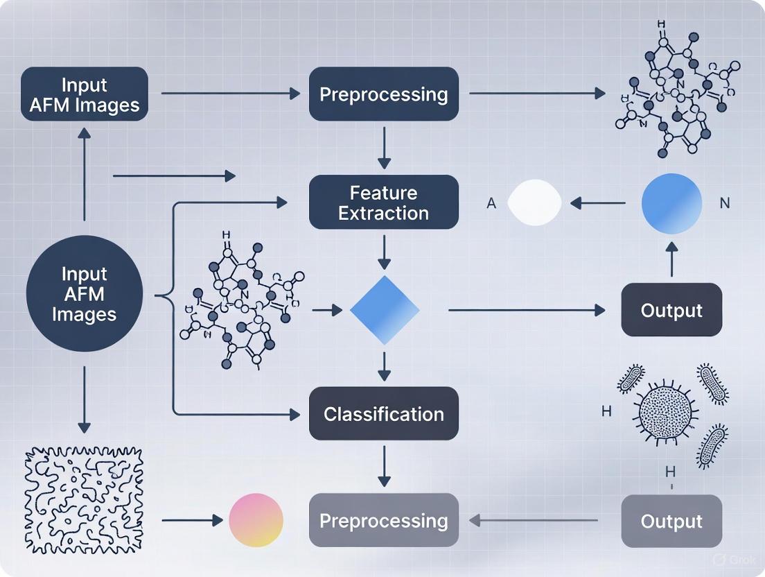
Figure 1: Machine learning workflow for AFM biofilm image analysis
Experimental Protocols for AFM Biofilm Imaging
Sample Preparation Methods
Proper sample preparation is critical for successful AFM imaging of biofilms while preserving their native structure. The following protocols have been validated for reliable biofilm characterization:
4.1.1 Substrate Selection and Functionalization
- Surface Treatment: Use PFOTS-treated glass coverslips or freshly cleaved mica to promote biofilm adhesion [1]. PFOTS (perfluorooctyltrichlorosilane) creates a hydrophobic surface that facilitates bacterial attachment while providing a smooth baseline for imaging.
- Alternative Functionalizations: (3-aminopropyl)triethoxysilane or NiCl₂-coated mica can be used, though these may cause flattening of structures or round artefacts during direct air-drying [5].
- Combinatorial Approaches: Gradient-structured surfaces allow simultaneous study of how varying surface properties influence attachment dynamics and community structure [1].
4.1.2 Biofilm Immobilization Techniques
- Mechanical Immobilization: Utilize porous membranes or polydimethylsiloxane (PDMS) stamps with customized microstructures (1.5-6 μm wide, 0.5 μm pitch, 1-4 μm depth) to physically trap microbial cells [2]. This approach offers secure immobilization capable of withstanding lateral forces during scanning.
- Chemical Immobilization: Apply poly-l-lysine, trimethoxysilyl-propyl-diethylenetriamine, or carboxyl group cross-linking to promote adhesion [2]. Optimization with divalent cations (Mg²⁺, Ca²⁺) and glucose may provide optimal attachment without significant reduction in viability [2].
- Liquid Cell Preparation: For hydrated imaging, use sample holders with integrated liquid baths (85 mm² area capacity) with up to 420 μl of appropriate biological solution [4]. Employ long tips (500-1000 μm) glued to the sensor's oscillating prong to allow partial submersion while maintaining sensor functionality.
4.1.3 Fixation and Dehydration for High-Resolution Imaging
- Optimal Preservation: Ethanol gradient dehydration followed by critical point drying best preserves native biofilm morphology [5].
- Alternative Method: Chemical dehydration with dimethoxypropane results in well-balanced shape distributions with lower aspect ratios [5].
- Fixation Importance: Chemical fixation plays a crucial role in both capturing and protecting biological structures on substrates, particularly for high-resolution imaging [5].
Imaging Parameters and Conditions
4.2.1 Instrument Configuration
- Sensor Selection: Employ stiff qPlus sensors (k ≥ 1 kN/m) for FM-AFM imaging in liquid environments, enabling small amplitude oscillation (<100 pm) and high sensitivity to short-range forces [4].
- Liquid Imaging: Maintain minimal penetration depth of the tip in liquid to preserve high Q factors (up to 1000 achievable) while ensuring sufficient immersion for biological relevance [4].
- Environmental Control: Conduct imaging at controlled temperature (typically 20-25°C) and humidity (40% recommended) to minimize evaporation effects during extended acquisitions [4].
4.2.2 Scanning Parameters
- Large-Area Imaging: Implement automated large-area AFM with limited overlap between adjacent scans (typically 5-10%) to maximize acquisition speed while maintaining image continuity [1].
- Resolution Settings: Configure pixel density to balance resolution and acquisition time; for overview scans, 512×512 pixels over 100×100 μm areas provides sufficient detail, while high-resolution cellular imaging may require 1024×1024 pixels over smaller regions [1].
- Force Control: Maintain minimal interaction forces (below 100 pN) to prevent damage to delicate biofilm structures, using frequency shift setpoints of -1 to -7 Hz in FM-AFM mode [4].
Figure 2: AFM biofilm imaging experimental workflow
Quantitative Analysis of Biofilm Properties
AFM enables comprehensive quantification of structural and mechanical properties essential for understanding biofilm function and response to interventions. The large-area automated approach combined with machine learning analysis facilitates statistically robust characterization across multiple scales.
Table 2: Quantitative Parameters Accessible Through AFM Biofilm Imaging
| Parameter Category | Specific Measurable Parameters | Biological Significance | Measurement Technique |
|---|---|---|---|
| Structural Properties | Cellular dimensions (length: ~2 μm, diameter: ~1 μm for Pantoea sp. YR343) [1] | Growth state, cell division | Topographical imaging |
| Flagellar dimensions (height: 20-50 nm, length: tens of μm) [1] | Motility, surface attachment | High-resolution AFM | |
| Spatial distribution patterns (honeycomb organization) [1] | Community architecture, cell-cell interactions | Large-area mapping | |
| Mechanical Properties | Elastic modulus via nanoindentation | Biofilm stiffness, structural integrity | Force spectroscopy |
| Adhesion forces (cell-surface and cell-cell) | Attachment strength, cohesion | Force-distance measurements | |
| Turgor pressure of encapsulated cells | Cell viability, metabolic state | Hertz model analysis [2] | |
| Dynamic Processes | Surface coverage and confluency | Biofilm development stage | ML-based segmentation |
| Cellular orientation and alignment | Response to surface properties | Vector analysis | |
| Roughness and topography evolution | Structural complexity development | 3D surface analysis |
Research Reagent Solutions for AFM Biofilm Studies
Table 3: Essential Materials and Reagents for AFM Biofilm Imaging
| Reagent/Material | Function/Application | Usage Notes |
|---|---|---|
| PFOTS (Perfluorooctyltrichlorosilane) | Surface treatment for glass substrates to promote bacterial adhesion | Creates hydrophobic surface; compatible with various bacterial species [1] |
| (3-Aminopropyl)triethoxysilane | Alternative surface functionalization for mica substrates | May cause flattening of biological structures [5] |
| NiCl₂ Coating | Mica functionalization for enhanced EV and bacterial capture | Prone to formation of round artefacts during direct air-drying [5] |
| Poly-L-Lysine | Chemical immobilization agent for microbial cells | Provides strong adhesion but may affect cell viability and nanomechanical properties [2] |
| Ethanol Gradient Series | Dehydration protocol for sample preservation | Critical for maintaining morphology; typically 30%-50%-70%-90%-100% series [5] |
| Critical Point Dryer | Sample drying equipment for morphology preservation | Superior to hexamethyldisilazane for retaining native structures [5] |
| PDMS Stamps | Mechanical immobilization with customized microstructures | Enables cell orientation control; dimensions customizable for target cells (1.5-6 μm wide, 0.5 μm pitch) [2] |
| Sapphire Tips | AFM probes for high-resolution imaging in liquid | Chemically inert, very hard; suitable for biological imaging [4] |
Case Study: Honeycomb Pattern Discovery in Pantoea sp. YR343
The power of large-area AFM combined with machine learning analysis is exemplified by the recent discovery of a unique honeycomb pattern in Pantoea sp. YR343 biofilms [1]. This case study demonstrates how advanced AFM methodologies can reveal previously unrecognized structural organizations in microbial communities.
Experimental Implementation: Researchers employed large-area automated AFM to image Pantoea sp. YR343 on PFOTS-treated glass surfaces during early attachment stages (30 minutes to 8 hours post-inoculation) [1]. The automated system captured high-resolution images across millimeter-scale areas, with machine learning algorithms processing over 19,000 individual cells to quantify spatial organization patterns [1] [3].
Key Findings: Analysis revealed that surface-attached cells exhibited a preferred cellular orientation, self-organizing into a distinctive honeycomb pattern with precisely regulated gaps between cell clusters [1]. High-resolution imaging enabled visualization of flagellar structures bridging these gaps, suggesting that flagellar coordination plays a role in biofilm assembly beyond initial attachment [1]. The identification of these structures as flagella was confirmed using a flagella-deficient control strain, which showed no similar appendages under AFM [1].
Biological Significance: Though the complete biological role of these patterns requires further investigation, researchers hypothesize they likely contribute to biofilm cohesion and adaptability by creating an interconnected network that facilitates nutrient transport, communication, and structural stability [3]. This organizational pattern would have remained undetected using conventional AFM approaches limited to small imaging areas.
The integration of atomic force microscopy with machine learning represents a transformative advancement in biofilm research, enabling comprehensive structural and mechanical characterization of these complex microbial communities at scales relevant to their natural environments [1]. The development of large-area automated AFM has successfully addressed the longstanding limitation of traditional AFM - the inability to connect nanoscale cellular features with broader community organization patterns [1] [3].
Future developments in AFM technology for biofilm research will likely focus on enhancing real-time imaging capabilities under physiologically relevant conditions, further expanding the scale of automated imaging, and refining machine learning algorithms for predictive modeling of biofilm development and treatment responses [1]. These advancements will provide increasingly powerful tools to address the significant challenges posed by biofilms in clinical, industrial, and environmental contexts, particularly in an era of escalating antimicrobial resistance [8].
As AFM technologies continue to evolve alongside machine learning and artificial intelligence, researchers will gain unprecedented capabilities to decipher the structural principles governing biofilm resilience and develop targeted strategies for biofilm control in healthcare and industrial applications [1] [7]. The combination of high-resolution imaging, nanomechanical property mapping, and large-scale architectural analysis positions AFM as an indispensable platform for advancing our fundamental understanding of biofilm biology and developing effective interventions against biofilm-associated challenges.
Atomic Force Microscopy (AFM) has emerged as a pivotal tool in biofilm research, capable of revealing structural and mechanical properties at the nanoscale. However, a significant challenge persists in linking these nanoscale observations to the functional macroscale organization of biofilms [1]. This application note addresses this scale-transition challenge through automated large-area AFM imaging coupled with machine learning (ML) classification, providing researchers with standardized protocols to bridge the resolution gap in microbial community analysis.
The inherent heterogeneity of biofilms—characterized by spatial and temporal variations in structure, composition, and density—necessitates advanced analytical approaches that can operate across multiple scales [1]. Traditional AFM methods, while providing critically important high-resolution insights, suffer from limited scan range and labor-intensive operation, restricting their ability to capture the full spatial complexity of biofilm architectures [1]. The integration of machine learning with expanded imaging capabilities now enables comprehensive characterization from cellular features to community-scale organization.
Quantitative Data Presentation
Performance Comparison: Human vs. Machine Learning Classification
Table 1: Classification accuracy for staphylococcal biofilm images
| Classification Method | Mean Accuracy | Recall | Off-by-One Accuracy |
|---|---|---|---|
| Human Researchers | 0.77 ± 0.18 | Not specified | Not specified |
| Machine Learning Algorithm | 0.66 ± 0.06 | Comparable to human | 0.91 ± 0.05 |
Evaluation of staphylococcal biofilm images against an established ground truth demonstrates that while human observers currently achieve higher mean accuracy, the developed ML algorithm provides robust classification with excellent off-by-one accuracy, indicating strong proximity to correct classifications [9]. This performance makes the algorithm suitable for high-throughput screening applications where consistency and scalability outweigh marginal accuracy differences.
AFM Imaging Specifications and Capabilities
Table 2: Technical specifications of AFM imaging approaches
| Parameter | Conventional AFM | Large Area Automated AFM |
|---|---|---|
| Maximum Scan Area | <100 µm | Millimeter-scale |
| Resolution | Nanoscale (sub-cellular) | Nanoscale to cellular |
| Cellular Feature Detection | Individual cells (~2 µm length) | Individual cells and flagella (20-50 nm height) |
| Flagellar Visualization | Limited | Detailed (~20-50 nm height) |
| Throughput | Low (labor-intensive) | High (automated) |
| Spatial Context | Limited local information | Comprehensive spatial heterogeneity |
Large area automated AFM significantly expands capability for biofilm analysis by capturing high-resolution images over millimeter-scale areas, enabling visualization of previously obscured spatial heterogeneity and cellular morphology during early biofilm formation [1]. This approach reveals organized cellular patterns, such as the distinctive honeycomb arrangement observed in Pantoea sp. YR343, and enables detailed mapping of flagellar interactions that play crucial roles in biofilm assembly beyond initial attachment [1].
Experimental Protocols
Large Area AFM Biofilm Imaging Protocol
Principle: Automated large-area AFM enables comprehensive analysis of microbial communities over extended surface areas with minimal user intervention, capturing both nanoscale features and macroscale organization [1].
Materials:
- Bacterial strain (e.g., Pantoea sp. YR343)
- PFOTS-treated glass coverslips or silicon substrates
- Appropriate liquid growth medium
- Atomic Force Microscope with large-area capability
- Image stitching software
- Machine learning-based image segmentation tools
Procedure:
- Surface Preparation: Treat glass coverslips with PFOTS to create standardized surfaces for bacterial attachment [1].
- Inoculation: Inoculate petri dish containing treated coverslips with bacterial cells in liquid growth medium.
- Incubation: Incubate under appropriate conditions for selected time points (e.g., ~30 minutes for initial attachment, 6-8 hours for cluster formation).
- Sample Harvesting: At each time point, remove coverslip from Petri dish and gently rinse to remove unattached cells.
- Sample Drying: Air-dry samples before imaging to preserve structural integrity.
- Automated AFM Imaging: Implement automated large-area scanning protocol with minimal overlap between adjacent images to maximize acquisition speed.
- Image Processing: Apply stitching algorithms to create seamless, high-resolution composite images from individual scans.
- Feature Extraction: Utilize ML-based segmentation for automated extraction of parameters including cell count, confluency, cell shape, and orientation.
- Spatial Analysis: Quantify spatial heterogeneity, cellular patterning, and appendage interactions across the imaged area.
Technical Notes:
- The limited overlap between scans maximizes acquisition speed while maintaining image continuity [1]
- ML-driven image segmentation manages high-volume, information-rich data efficiently
- The method enables quantitative analysis of microbial community characteristics over extensive areas
- High-resolution capability allows visualization of flagellar structures measuring ~20-50 nm in height and extending tens of micrometers across surfaces
Machine Learning Classification Protocol for Biofilm Maturity
Principle: A machine learning algorithm can classify biofilm maturity based on topographic characteristics identified by AFM, independent of incubation time, using a predefined framework of six distinct classes [9].
Materials:
- AFM images of staphylococcal biofilms
- Ground truth classification dataset
- Open access desktop tool for ML classification
- Computational resources for algorithm training/execution
Procedure:
- Image Acquisition: Collect AFM images of staphylococcal biofilms using standardized imaging parameters.
- Feature Identification: Define characteristic topographic features including substrate properties, bacterial cells, and extracellular matrix components.
- Ground Truth Establishment: Create reference classification based on the six-class framework by expert consensus.
- Algorithm Training: Train ML algorithm to recognize pre-set characteristics of biofilms corresponding to different maturity classes.
- Validation: Compare algorithm performance against ground truth using accuracy, recall, and off-by-one accuracy metrics.
- Classification: Implement trained algorithm to classify new AFM images into the six maturity classes.
- Output Analysis: Interpret results in context of biofilm development stage and structural properties.
Technical Notes:
- The six-class framework is based on common topographic characteristics rather than temporal development [9]
- Human observers achieve mean classification accuracy of 0.77 ± 0.18 [9]
- ML algorithm achieves mean accuracy of 0.66 ± 0.06 with off-by-one accuracy of 0.91 ± 0.05 [9]
- The approach circumvents observer bias and enables high-throughput analysis
- Open access desktop tool availability promotes method standardization
Workflow Visualization
Biofilm Analysis Workflow
ML Classification Process
Research Reagent Solutions
Table 3: Essential materials and reagents for AFM biofilm research
| Reagent/Material | Specification | Function/Application |
|---|---|---|
| Pantoea sp. YR343 | Gram-negative rhizosphere bacterium | Model organism for biofilm assembly studies |
| PFOTS-treated surfaces | Trichloro(1H,1H,2H,2H-perfluorooctyl)silane | Standardized hydrophobic surfaces for bacterial attachment |
| Silicon substrates | Various surface modifications | Testing surface property effects on bacterial adhesion |
| Staphylococcal strains | Clinical isolates | Biofilm maturity classification studies |
| ML Classification Tool | Open access desktop software | Automated classification of biofilm images |
| Image Stitching Algorithm | Custom-developed with minimal feature matching | Seamless composite image creation from multiple scans |
| AFM with large-area capability | Automated scanning system | Millimeter-scale high-resolution imaging |
The recommended research reagents support comprehensive biofilm analysis from initial attachment to mature community formation. Pantoea sp. YR343 serves as an excellent model organism due to its well-characterized biofilm-forming capabilities, peritrichous flagella, and distinctive honeycomb patterning during surface colonization [1]. PFOTS-treated surfaces provide consistent hydrophobic substrates for reproducible attachment studies, while variable silicon substrates enable investigation of surface property effects on biofilm assembly [1].
The open access ML classification tool represents a significant advancement for standardized biofilm maturity assessment, enabling researchers to bypass labor-intensive manual classification while maintaining analytical rigor [9]. Combined with large-area AFM capabilities, these reagents create an integrated workflow for multiscale biofilm characterization.
The integration of machine learning (ML) with Atomic Force Microscopy (AFM) is revolutionizing the quantitative analysis of bacterial biofilms. AFM provides unparalleled high-resolution topographical and nanomechanical data at the cellular and sub-cellular level, but traditional analysis methods struggle to efficiently process the vast, information-rich datasets generated, especially with the advent of large-area automated AFM that captures images over millimeter-scale areas [1]. This application note details the core ML paradigms—supervised and unsupervised learning—for extracting meaningful, quantitative information from AFM biofilm images, framed within the context of a broader thesis on ML classification in this field. We provide structured comparisons, detailed experimental protocols, and essential resource toolkits tailored for researchers, scientists, and drug development professionals.
Core ML Paradigms in Biofilm Analysis
The choice between supervised and unsupervised learning is dictated by the research question and the availability of annotated training data. The table below summarizes the primary applications of each paradigm in the context of AFM biofilm image analysis.
Table 1: Comparison of Supervised and Unsupervised Learning for AFM Biofilm Data Analysis
| Feature | Supervised Learning | Unsupervised Learning |
|---|---|---|
| Primary Use Case | Classification, Object Detection, Segmentation | Exploratory Data Analysis, Feature Reduction, Domain Segmentation |
| Required Input Data | Labeled AFM images (e.g., biofilm maturity classes, cell annotations) | Raw, unlabeled AFM image data |
| Key Outputs | Predictive model for classifying new images, detection of specific features | Identification of inherent patterns, clusters, or data structures |
| Example Applications | - Classifying biofilm maturity stages [9]- Detecting and counting individual cells [1]- Segmenting cells from the background or EPS | - Identifying polymer domains in blend films [10]- Reducing feature dimensions for downstream analysis |
| Advantages | High accuracy for well-defined tasks; directly addresses specific hypotheses | No need for labor-intensive labeling; can reveal unexpected patterns |
| Disadvantages | Requires large, high-quality labeled datasets; prone to bias in training data | Results can be more abstract and require expert interpretation |
Supervised Learning: Protocols and Applications
Biofilm Maturity Classification
Objective: To train a model that automatically classifies AFM images of staphylococcal biofilms into predefined maturity stages based on topographic features [9].
Experimental Protocol:
- Image Acquisition: Acquire AFM images of biofilms (e.g., Staphylococcus strains) grown under controlled conditions for varying durations.
- Ground Truth Labeling: Manually label each image into one of six maturity classes (e.g., Class 1: Substrate with isolated cells; Class 6: Complex 3D structures fully embedded in matrix) based on established topographic characteristics [9].
- Data Preprocessing:
- Image Stitching: For large-area AFM, use automated stitching algorithms to create a seamless, high-resolution mosaic from individual scans [1].
- Augmentation: Apply transformations (e.g., rotation, flipping, minor contrast adjustments) to the training dataset to improve model robustness.
- Model Training & Evaluation:
- Framework: Develop a convolutional neural network (CNN) or utilize a pre-trained network (ResNet) with transfer learning.
- Training: Train the model on the augmented dataset of labeled images.
- Performance Metrics: Evaluate model performance using accuracy, recall, and "off-by-one" accuracy (which tolerates a one-class error), comparing it to human expert classification (e.g., human accuracy: 0.77 ± 0.18; model accuracy: 0.66 ± 0.06) [9].
Single-Cell Detection and Morphological Analysis
Objective: To automatically identify and segment individual bacterial cells in large-area AFM images to quantify parameters like cell count, confluency, shape, and orientation [1].
Experimental Protocol:
- Image Acquisition: Collect large-area AFM scans of early-stage biofilms (e.g., Pantoea sp. YR343) where cells are distinctly separated [1].
- Data Annotation: Manually annotate the boundaries of individual cells in the images to create ground truth data for training. Tools like Computer Vision Annotation Tool (CVAT) can be used for this purpose [11].
- Model Training:
- Quantitative Analysis: Use the model's output to extract quantitative data, such as the discovery of a preferred cellular orientation forming a honeycomb pattern in Pantoea sp. YR343 [1].
The following diagram illustrates the typical workflow for a supervised learning project in this domain.
Unsupervised Learning: Protocols and Applications
Self-Supervised Learning for Low-Data Regimes
Objective: To classify biofilm image components (cells, microbial byproducts, non-occluded surface) with high accuracy using minimal expert-annotated data [12].
Experimental Protocol:
- Image Preprocessing: Apply Contrast Limited Adaptive Histogram Equalization (CLAHE) to sharpen features in SEM/AFM images. Use super-resolution models to enhance image resolution and reduce shape variations [12].
- Patch Generation: Divide each biofilm image into a large number of smaller patches. These patches form the unlabeled dataset for the initial training phase.
- Self-Supervised Pre-training: Train a model (e.g., using Barlow Twins or MoCoV2 framework) on the unlabeled patches to learn powerful representations of the underlying image data without any manual labels [12].
- Supervised Fine-tuning: Fine-tune the pre-trained model on a small subset (~10%) of expert-annotated image patches labeled as "cells," "byproducts," or "non-occluded surface." This step adapts the general representations to the specific classification task [12].
- Model Deployment: Use the fine-tuned model to classify patches in new images and generate distribution heatmaps for each component, achieving high accuracy with a fraction of the annotation effort [12].
Domain Segmentation in AFM Images
Objective: To identify distinct polymer domains within AFM images of polymer blends with minimal manual intervention, qualifying the phase separation state [10].
Experimental Protocol:
- Feature Extraction: For each AFM image, compute features using Discrete Fourier Transform (DFT) or Discrete Cosine Transform (DCT) to capture spatial frequency information.
- Clustering: Apply unsupervised clustering algorithms (e.g., K-means) on the extracted features (e.g., variance statistics) to group image regions into distinct domains [10].
- Post-processing: Use image processing libraries like the Porespy Python package to calculate the size distribution of the identified domains from the segmented image, which helps qualify the material's phase-separated state [10].
The Scientist's Toolkit: Research Reagent Solutions
Table 2: Essential Research Reagents, Tools, and Software for ML-Based AFM Biofilm Analysis
| Item Name | Function/Application | Relevant Protocol |
|---|---|---|
| PFOTS-Treated Glass | Creates a hydrophobic surface to study specific bacterial adhesion and early biofilm formation dynamics [1]. | Large-Area AFM of Pantoea sp. |
| Computer Vision Annotation Tool (CVAT) | Open-source, web-based tool to manually annotate images for creating ground truth data for supervised learning [11]. | Single-Cell Detection |
| Porespy Python Package | A toolkit for the analysis of porous media images, used for calculating domain size distributions from segmented images [10]. | Unsupervised Domain Segmentation |
| OpenCV Python Library | Provides classical computer vision algorithms (e.g., blob detection, thresholding) for unsupervised pre-annotation and image preprocessing [11]. | Self-Supervised Learning |
| Barlow Twins / MoCoV2 Models | Self-supervised learning frameworks for learning powerful image representations from unlabeled data, minimizing expert annotation needs [12]. | Self-Supervised Learning |
| Large-Area Automated AFM | An advanced AFM system capable of automated, high-resolution scanning over millimeter-scale areas, generating comprehensive datasets for ML analysis [1]. | All Protocols |
| Mask R-CNN Model | A state-of-the-art deep learning architecture for instance segmentation, used for detecting and outlining individual cells in an image [11]. | Single-Cell Detection |
Atomic Force Microscopy (AFM) provides high-resolution, nanoscale insights into the structural and functional properties of bacterial biofilms, capturing details from individual cells to extracellular matrix components [1]. The inherent heterogeneity and dynamic nature of biofilms, characterized by spatial and temporal variations in structure and composition, present a significant challenge for consistent analysis [1] [13]. Machine learning (ML) is transforming this field by automating the classification of biofilm maturity and morphology, overcoming the limitations of manual evaluation which is time-consuming and subject to observer bias [9]. This document outlines standardized protocols and application notes for employing ML in the classification of AFM biofilm images, framed within the broader objective of developing robust, automated tools for biofilm research and therapeutic intervention.
Application Notes: Machine Learning in AFM Biofilm Analysis
The integration of ML with AFM imaging addresses critical bottlenecks in biofilm research, enabling high-throughput, quantitative analysis of complex image data.
- Automated Classification of Biofilm Maturity: A key application is the classification of biofilm maturity stages independent of incubation time. One established framework defines six distinct classes based on topographic characteristics observed in AFM, such as the substrate coverage, bacterial cells, and extracellular matrix [9]. While human experts can classify images with a mean accuracy of 0.77 ± 0.18, a dedicated ML algorithm can achieve a mean accuracy of 0.66 ± 0.06. Notably, the algorithm's "off-by-one" accuracy of 0.91 ± 0.05 indicates it rarely misclassifies a biofilm into a non-adjacent maturity stage, demonstrating its reliability for screening purposes [9].
- Enhanced Analysis via Large-Area AFM: Traditional AFM is limited by small scan areas (<100 µm), making it difficult to link nanoscale features to the biofilm's macroscopic architecture [1]. Large-area automated AFM, combined with ML, overcomes this by capturing high-resolution images over millimeter-scale areas. Machine learning aids in seamless stitching of these images, cell detection, and classification, revealing previously obscured spatial heterogeneities and patterns, such as a preferred cellular orientation in Pantoea sp. YR343 biofilms [1].
- Identification of Species-Specific Patterns: The high resolution of AFM allows for the visualization of species-specific features critical for understanding early biofilm formation. For instance, AFM can clearly resolve flagellar structures (~20–50 nm in height) and their coordination during the surface attachment of Pantoea sp. YR343 [1]. ML models can be trained to recognize these and other fine features, such as pili or the honeycomb-like patterns formed by cell clusters, enabling the identification of morphological signatures specific to bacterial species or strains [1].
Table 1: Performance Metrics of a Machine Learning Algorithm for Classifying Staphylococcal Biofilm Maturity [9]
| Metric | Human Expert Performance | Machine Learning Algorithm Performance |
|---|---|---|
| Mean Accuracy | 0.77 ± 0.18 | 0.66 ± 0.06 |
| Recall | Not Specified | Comparable to human performance |
| Off-by-One Accuracy | Not Specified | 0.91 ± 0.05 |
Table 2: Essential Research Reagent Solutions for AFM-Based Biofilm Studies
| Item | Function / Application |
|---|---|
| Pantoea sp. YR343 | A model gram-negative, rod-shaped bacterium with peritrichous flagella and pili for studying early attachment dynamics and honeycomb pattern formation [1]. |
| PFOTS-Treated Glass Surfaces | Creates a hydrophobic substrate to study the effects of surface properties on initial bacterial adhesion and biofilm assembly [1]. |
| Open Access ML Classification Tool | A desktop software tool designed to identify pre-set topographic characteristics and classify AFM biofilm images into pre-defined maturity classes [9]. |
Experimental Protocols
Protocol 1: ML-Assisted Classification of Biofilm Maturity Based on Topographic Classes
This protocol is adapted from research on staphylococcal biofilms [9].
Biofilm Growth and AFM Imaging:
- Grow biofilms on relevant substrates (e.g., glass, plastic) under controlled conditions.
- At desired time points, rinse the substrate gently to remove non-adherent cells.
- Acquire topographic images of the biofilms using Atomic Force Microscopy (AFM). Ensure images capture key features: the substrate, individual bacterial cells, and the extracellular matrix.
Ground Truth Establishment:
- Assemble a set of AFM biofilm images.
- Have a group of independent, trained researchers manually classify each image into one of the six predefined maturity classes based on topographic characteristics [9]. This classified set establishes the ground truth for model training.
Machine Learning Model Training:
- Extract features from the AFM images (e.g., texture, height distribution, surface roughness).
- Train a supervised machine learning algorithm (e.g., a convolutional neural network) using the ground-truthed image set.
- Validate the model using a separate test set of images. The model should be capable of discriminating between the six different classes with performance metrics targeting an accuracy near 0.66 and an off-by-one accuracy exceeding 0.90 [9].
Deployment and Analysis:
- Use the trained model to classify new, unlabeled AFM biofilm images.
- The open-access desktop tool referenced in the research can be employed for this task [9].
Protocol 2: Probing Early Biofilm Assembly Using Large-Area Automated AFM
This protocol is adapted from studies on Pantoea sp. YR343 [1].
Surface Preparation and Inoculation:
- Prepare PFOTS-treated glass coverslips to create a uniform, hydrophobic surface.
- Inoculate a Petri dish containing the treated coverslips with a liquid culture of the bacterial strain of interest (e.g., Pantoea sp. YR343).
Sample Harvesting and Preparation:
- At selected early time points (e.g., 30 minutes, 6-8 hours), remove a coverslip from the Petri dish.
- Gently rinse the coverslip with a buffer solution to remove unattached, planktonic cells.
- Air-dry the sample prior to AFM imaging.
Large-Area Automated AFM Imaging:
- Mount the sample on an automated large-area AFM.
- Program the system to capture multiple, contiguous high-resolution scans over a millimeter-scale area of the surface.
- Use machine learning algorithms to automatically stitch the individual images into a seamless, large-area topographic map [1].
Image Analysis and Feature Extraction:
- Apply ML-based segmentation to the stitched large-area image to identify individual cells.
- Automate the extraction of quantitative parameters, including cell count, surface confluency, cell shape, and cellular orientation [1].
- Visually inspect the high-resolution map for fine features like flagella and the organization of cell clusters.
Workflow Visualization
Implementing ML Models for AFM Biofilm Analysis: Techniques and Workflows
Atomic Force Microscopy (AFM) is a powerful tool for high-resolution topographical imaging of biofilms, enabling the study of their structural development and response to treatments at the nanoscale [1]. Traditional manual analysis of AFM images is time-consuming, subjective, and prone to human bias [9] [14] [15]. While machine learning (ML) offers potential for automated analysis, researchers often face the significant challenge of data scarcity, with limited experimentally obtained AFM images available for training robust models [15].
This Application Note provides a structured guide to ML strategies that address the small dataset problem in AFM biofilm image analysis. We detail specific protocols and evaluate the performance of different approaches, enabling researchers to select and implement appropriate methods for their specific research contexts.
The following strategies have been successfully applied to overcome data scarcity in AFM-based biofilm studies. Their key characteristics and reported performance are summarized in the table below.
Table 1: Performance Comparison of ML Strategies for Small AFM Datasets
| Strategy | Reported Accuracy/Performance | Key Advantages | Ideal Use Case |
|---|---|---|---|
| Unsupervised Feature Engineering (DFT/DCT) | Outperformed ResNet50 in segmentation task [15] | No manual labeling; interpretable features; works on small N | Domain segmentation in polymer blends [15] |
| Classical Supervised Learning | Mean accuracy: 0.66 ± 0.06; Recall: comparable to human; Off-by-one accuracy: 0.91 ± 0.05 [9] [14] | Leverages expert knowledge via labeling; more efficient training | Biofilm maturity classification [9] [14] |
| Convolutional Neural Networks (CNN) | Enabled prediction of electrochemical impedance spectra from AFM images [16] | High feature detection capability; can use pre-trained models | Defect detection and coordinate mapping [16] |
| Data Augmentation | Used in training a model for 6-class biofilm classification [14] | Artificially expands dataset size from limited original images | All supervised learning approaches, particularly with deep learning |
Detailed Methodologies and Protocols
Unsupervised Learning with Signal Processing Features
This approach is ideal for tasks like segmenting different domains within a biofilm (e.g., cells, extracellular polymeric substance (EPS), substrate) without the need for extensive labeled data.
Protocol: Domain Segmentation using Discrete Fourier Transform (DFT)
- Image Pre-processing: Convert AFM images to grayscale if necessary. Apply a Gaussian blur (σ = 1.0) to reduce high-frequency noise [15].
- Feature Extraction using DFT:
- For each image, compute the 2D Discrete Fourier Transform (DFT).
- Calculate the variance of the magnitude of the DFT coefficients within a sliding window (e.g., 16x16 pixels) across the image. This variance acts as a texture descriptor that distinguishes different domains [15].
- Reshape the resulting feature map into a feature vector for each pixel or image region.
- Clustering: Apply an unsupervised clustering algorithm, such as K-means, to the feature vectors to group image regions with similar textural properties. The number of clusters (K) should correspond to the expected number of domains (e.g., substrate, cells, EPS) [15].
- Post-processing: Use morphological operations, such as opening and closing, to smooth the resulting segmentation mask and remove small noise-induced artifacts [15].
Supervised Learning with Expert-Defined Classes
This protocol is based on a study that classified staphylococcal biofilms into six maturity levels using a limited dataset of 138 unique AFM images [9] [14].
Protocol: Biofilm Maturity Classification
- Define a Classification Framework:
- Establish clear, objective classes based on quantifiable AFM image characteristics. The example framework uses the percentage coverage of three characteristics [14]:
- Implant material (substrate)
- Bacterial cells
- Extracellular matrix (ECM)
- Example Class Definitions [14]:
- Class 0: 100% substrate, 0% cells, 0% ECM.
- Class 1: 50-100% substrate, 0-50% cells, 0% ECM.
- Class 2: 0-50% substrate, 50-100% cells, 0% ECM.
- Class 3: 0% substrate, 50-100% cells, 0-50% ECM.
- Class 4: 0% substrate, 0-50% cells, 50-100% ECM.
- Class 5: 0% substrate, cells not identifiable, 100% ECM.
- Establish clear, objective classes based on quantifiable AFM image characteristics. The example framework uses the percentage coverage of three characteristics [14]:
- Annotation and Ground Truth Establishment:
- Manually annotate the AFM image dataset according to the defined framework. Using a 10x10 grid overlaid on each image can help consistently estimate percentage coverages [14].
- To ensure reliability, have multiple independent researchers classify a test set of images and calculate inter-observer variability. Human observers achieved a mean accuracy of 0.77 ± 0.18 in one study, validating the framework [9] [14].
- Dataset Preparation and Augmentation:
- Model Training and Evaluation:
- Train a machine learning model (e.g., a deep learning algorithm) on the augmented training set. The model should be appropriately sized for the available data to prevent overfitting.
- Evaluate the model on the held-out test set. Report key metrics beyond accuracy, such as recall and precision, especially since class imbalance is common. The referenced model achieved a mean accuracy of 0.66 ± 0.06 and a high off-by-one accuracy of 0.91 ± 0.05, indicating it rarely made large classification errors [9] [14].
CNN for Defect Detection and Coordinate Mapping
For tasks requiring precise localization of features (e.g., pores in a membrane, individual cells), a CNN-based object detector can be used, even with smaller datasets.
Protocol: Defect Coordinate Detection with CNN
- Data Preparation and Annotation:
- Annotate AFM images by marking the center coordinates (X, Y) and the approximate radius of each target defect or cell [16].
- These coordinates are used to define bounding boxes for each object.
- Model Selection and Training:
- Employ a Convolutional Neural Network (CNN) architecture designed for object detection, such as a Region-Based CNN (R-CNN) or a variant like Cascade Mask-RCNN, which has been used for nanoparticle detection in microscopy images [16].
- Train the CNN to detect the bounding boxes of the defects. The model learns to identify the unique topographical features associated with the defects in the AFM images.
- Validation and Downstream Analysis:
- Validate detection accuracy by comparing predicted defect coordinates against the manual ground truth, using metrics like precision and recall [16].
- The output coordinates can be used for further analysis, such as calculating defect density, spatial distribution (e.g., via Voronoi tessellation), or as input for finite element modeling to predict functional properties like electrochemical impedance [16].
Diagram 1: A strategic workflow for applying machine learning to small AFM image datasets, outlining the main approaches and methods to overcome data scarcity.
The Scientist's Toolkit
Table 2: Essential Research Reagents and Computational Tools
| Item / Software | Function / Application | Notes |
|---|---|---|
| JPKSPM Data Processing | AFM image capture and processing | Used for initial image processing and cleaning [14]. |
| Titanium Alloy Discs (TAV, TAN) | Abiotic substrate for in vitro biofilm growth | Provides a standardized surface for implant-associated biofilm models [14]. |
| Glutaraldehyde (0.1% v/v) | Fixation of biofilm samples | Preserves biofilm structure for AFM imaging [14]. |
| Python with SciKit-Learn | Implementation of ML models and traditional algorithms | Primary environment for building custom unsupervised and supervised workflows [15]. |
| Porespy Python Package | Quantification of domain size distribution | Used for analysis after segmentation [15]. |
| Open Access Desktop Tool | Automated classification of biofilm AFM images | Example of a deployed tool from a research study [9] [14]. |
Evaluation Metrics for Imbalanced Data
When working with small and often imbalanced datasets, selecting the right evaluation metrics is critical. Accuracy can be misleading if one class is dominant [17] [18].
- Precision: Answers "What fraction of positive predictions are correct?" Important when the cost of false positives (false alarms) is high. Precision = TP / (TP + FP) [17] [18].
- Recall (True Positive Rate): Answers "What fraction of actual positives did we find?" Crucial when missing a positive (false negative) is costly. Recall = TP / (TP + FN) [17] [18].
- F1 Score: The harmonic mean of precision and recall. Provides a single metric that balances both concerns, especially useful for imbalanced datasets [17].
These metrics provide a more nuanced view of model performance than accuracy alone and should be reported alongside any classification results [17] [18].
The analysis of Atomic Force Microscopy (AFM) images of biofilms presents a significant challenge in microbiological research. While deep learning has gained prominence for image-based classification, alternative machine learning models—specifically decision trees and regression models—offer distinct advantages, including interpretability, lower computational resource requirements, and effectiveness with smaller datasets. These characteristics are vital for research environments where data may be limited and model transparency is essential for scientific validation. This document provides detailed application notes and protocols for integrating these classical machine learning techniques into a robust classification pipeline for AFM biofilm images, framed within a broader thesis on machine learning classification of AFM biofilm images research.
AFM is a powerful tool that functions as a translatable force gauge equipped with a nanometer-diameter sensing probe, capable of yielding nanometer-level detail about the surface of biological structures [19]. Its application in biofilm research is particularly valuable, as it allows for the in-situ determination of the mechanical properties of bacteria under genuine physiological liquid conditions, often without the need for external immobilization protocols that could denature the cell interface [20]. This capability is crucial for understanding dynamic phenomena of fundamental interest, such as biofilm formation and the dynamic properties of bacteria [20]. Recent advancements in High-Speed AFM (HS-AFM) further push the boundaries, but also introduce challenges in correct feature assignment for highly dynamic samples due to the interplay between the instrument's intrinsic sampling rate and the sample's internal redistribution rate [19]. The integration of machine learning, particularly interpretable models, is poised to deconvolute these complexities and extract meaningful biological insights from AFM data.
Theoretical Foundation and Rationale
The Case for Decision Trees and Regression in AFM Analysis
Decision trees and regression models provide a fundamentally different approach to pattern recognition compared to deep learning. Decision trees learn a series of hierarchical, binary decisions based on input features to arrive at a classification or prediction. This structure makes the model's decision logic transparent and easily interpretable, allowing researchers to understand which features in an AFM image (e.g., surface roughness, adhesion force, specific morphological traits) are most discriminative for classifying different biofilm states or bacterial types.
Regression models, particularly logistic regression for classification tasks, provide a statistical framework for understanding the relationship between a set of independent variables (image features) and a dependent variable (the biofilm class). The output of logistic regression includes coefficients for each feature, offering direct insight into the magnitude and direction of each feature's influence on the classification outcome. This aligns with the needs of scientific discovery, where understanding causal relationships and contributing factors is as important as the prediction itself.
The application of these models is particularly apt given the nature of AFM data. For instance, AFM can simultaneously acquire topographical data and mechanical properties like Young's modulus and turgor pressure [20]. These quantitative measurements are ideal, structured inputs for decision trees and regression models, which can efficiently learn the complex, often non-linear, relationships between these physical properties and biofilm phenotypes.
Comparative Analysis of Machine Learning Approaches for AFM
Table 1: Comparison of Machine Learning Models for AFM Biofilm Image Classification
| Model Characteristic | Deep Learning (e.g., CNNs) | Decision Trees/Random Forests | Regression Models (Logistic) |
|---|---|---|---|
| Interpretability | Low ("black box") | High (clear decision rules) | High (feature coefficients) |
| Data Efficiency | Requires large datasets (>>1000s of images) | Effective with small to medium datasets | Effective with small to medium datasets |
| Computational Demand | High (GPUs often essential) | Low to Moderate (CPU sufficient) | Low |
| Primary Input | Raw pixel data | Extracted features (e.g., texture, mechanics) | Extracted features (e.g., texture, mechanics) |
| Handling of Mixed Data | Poor (requires pre-processing) | Excellent (can handle numerical and categorical) | Good (requires encoding for categorical) |
| Typical Application | End-to-end image classification | Feature-based classification & insight generation | Feature importance analysis & probabilistic classification |
Experimental Protocols
Protocol 1: AFM Image Acquisition of Biofilms
Objective: To acquire high-quality, quantitative topographical and mechanical data from live biofilms under physiological conditions for subsequent machine learning analysis.
Materials:
- AFM System: A High-Speed AFM or a microscope capable of operating in force-volume or peak force tapping mode is recommended for dynamic samples [19] [20].
- Probes: Sharp, cantilevers with nominal spring constants appropriate for biological samples in liquid (e.g., 0.01-0.1 N/m).
- Bacterial Strain: The biofilm-forming strain of interest (e.g., Staphylococcal epidermidis, Staphylococcal aureus, Pseudomonas aeruginosa [21]).
- Growth Substrate: An appropriate, sterile solid substrate (e.g., glass slide, polycarbonate membrane, or textured biomaterial [21]).
- Physiological Liquid Medium: The appropriate sterile growth medium for the chosen bacterium (e.g., MM medium for Rhodococcus wratislaviensis [20]).
Procedure:
- Sample Preparation: Grow biofilms on the chosen substrate under controlled conditions relevant to your research question (e.g., temperature, time, nutrient availability). For live imaging, avoid chemical immobilization agents like poly-L-lysine, which can affect cell viability and surface properties [20]. Instead, utilize gentle preparation processes or leverage the bacterium's natural adhesion.
- AFM Calibration: Calibrate the AFM cantilever's sensitivity and spring constant following the manufacturer's established protocols.
- Imaging Parameter Setup:
- Scan Size: Set
[x_max, y_max]to encompass a representative area of the biofilm, typically several micrometers [19]. - Sampling/Pixilation: Set the pixel resolution. For a balance between resolution and speed, aim for a pixel size
(x_pixel, y_pixel)close to the tip diameterϕ. This provides the "maximum data driven image pixilation" [19]. The lateral scan rateυ_xcan be derived fromυ_x = f * ϕ, wherefis the oscillation frequency [19]. - Imaging Mode: Use a mode that minimizes lateral forces to avoid displacing the biofilm. Force-volume mode or high-speed versions of amplitude/frequency modulation (tapping mode) are suitable [19] [20].
- Scan Size: Set
- Data Acquisition: Acquire multiple images from different, independent biofilm samples. Simultaneously record height data and another channel, such as adhesion or deformation, if available.
- Data Export: Export image data in a format that preserves quantitative height information (e.g., .xyz, .tiff). Ensure metadata (scan size, setpoint, etc.) is recorded.
Protocol 2: Feature Extraction from AFM Image Data
Objective: To convert raw AFM image data into a set of quantitative descriptors (features) that characterize the biofilm's physical and morphological properties.
Materials:
- Software: Image analysis software (e.g., Gwyddion, GXLFM, or custom scripts in Python/MATLAB).
- Computing Environment: A standard laboratory computer.
Procedure:
- Image Pre-processing: Level the AFM images by mean plane subtraction to remove sample tilt. Use careful, minimal filtering to remove scan line noise without altering genuine surface features.
- Feature Calculation: For each AFM image (or defined regions of interest within an image), calculate a suite of quantitative features. These can be broadly categorized as follows:
- Topographical Features: Root-mean-square roughness (Rq), arithmetic average roughness (Ra), skewness, kurtosis, maximum peak height, maximum pit depth.
- Morphological Features: Surface area ratio, porosity, feature density, and grain size distribution (if applicable).
- Mechanical Features (from force curves): If force-volume data was acquired, extract Young's modulus and turgor pressure by fitting the retraction curve with appropriate mechanical models (e.g., Hertzian, Sneddon) [20].
- Data Structuring: Compile all extracted features for each image/region into a single table (DataFrame) where each row represents a sample and each column represents a feature. This table is the input for machine learning models.
Protocol 3: Model Training and Validation for Classification
Objective: To train and validate decision tree and logistic regression models for classifying biofilm images based on the extracted features.
Materials:
- Software: Python with scikit-learn, pandas, and numpy libraries, or equivalent statistical software (R, MATLAB).
- Dataset: The feature table from Protocol 2, with each sample assigned a class label (e.g., "Treatment" vs. "Control", "Strain A" vs. "Strain B").
Procedure:
- Data Preparation: Split the feature table into a training set (e.g., 70-80%) and a hold-out test set (e.g., 20-30%). Standardize the features by removing the mean and scaling to unit variance using the
StandardScalerfrom scikit-learn, fitting it only on the training data. - Model Training (Logistic Regression):
- Instantiate a
LogisticRegressionmodel. For datasets with suspected feature correlation, usepenalty='l1'(Lasso) to perform feature selection. - Train the model on the scaled training data using the
.fit()method.
- Instantiate a
- Model Training (Decision Tree/Random Forest):
- Instantiate a
DecisionTreeClassifierorRandomForestClassifier. The latter, being an ensemble of trees, generally provides better performance and robustness. - Train the model on the (unscaled) training data.
- Instantiate a
- Model Validation: Use k-fold cross-validation (e.g., k=5 or 10) on the training set to tune hyperparameters (e.g.,
Cfor regression,max_depthfor trees). Apply the final model to the hold-out test set to obtain an unbiased estimate of performance using metrics like accuracy, precision, recall, F1-score, and the area under the ROC curve (AUC-ROC). - Interpretation:
- For Logistic Regression, examine the magnitude and sign of the coefficients in the trained model. The largest absolute values indicate the most important features for classification.
- For Decision Trees/Random Forests, use the
feature_importances_attribute to rank the contribution of each input feature to the model's predictive power.
Data Presentation and Visualization
The Scientist's Toolkit: Essential Research Reagents and Materials
Table 2: Key Research Reagent Solutions for AFM-ML Biofilm Studies
| Item | Function/Application in Protocol |
|---|---|
| Poly[bis(octafluoropentoxy) phosphazene] (OFP) | A fluorinated biomaterial used to create smooth or textured surfaces with reduced bacterial adhesion, serving as a standardized substrate for studying biofilm resistance [21]. |
| Textured Substrates (500/500/600 nm pillars) | Surfaces with ordered submicron topography (diameter/spacing/height) fabricated via soft lithography; used to study the impact of surface patterning on bacterial adhesion and biofilm formation [21]. |
| Poly-L-lysine | A chemical immobilization agent. Note: Its use is discouraged for live-cell imaging as it can affect cell viability and surface properties, but it may be relevant for fixed-sample control studies [20]. |
| Isopore Polycarbonate Membranes | Used for mechanical entrapment of spherical cells for AFM imaging, an alternative to chemical immobilization, though it may impose mechanical stress [20]. |
| HS-AFM UGOKU Software | A freely available graphical user interface-based software package designed to assist with calculations related to feature assignment and experimental setup in HS-AFM studies of dynamic surfaces [19]. |
Workflow and Model Interpretation Diagrams
Diagram 1: AFM-ML Biofilm Analysis Workflow
Diagram 2: Decision Tree for Biofilm Classification
Atomic Force Microscopy (AFM) has been transformed from a tool for imaging nanoscale features into one that captures large-scale biological architecture. Traditional AFM, while powerful, has been fundamentally limited by its narrow field of view, making it difficult to understand how individual cellular features fit into larger organizational structures within biofilms. This limitation has been overcome through the development of an automated large-area AFM platform, which connects detailed observations at the level of individual bacterial cells with broader views covering millimeter-scale areas. This technological advance offers an unprecedented view of biofilm organization, with significant innovations for medicine, industrial applications, and environmental science.
The integration of this automated approach with machine learning represents a paradigm shift in biofilm research. Previously, researchers could examine individual bacterial cells in detail but not how they organize and interact as communities. The new platform changes this dynamic, enabling visualization of both the intricate structures of single cells and the larger patterns across entire biofilms. This capability is crucial for understanding how organisms interact with materials—a key step in identifying surface properties that resist biofilm formation, with important applications ranging from healthcare to food safety.
Experimental Protocols and Workflows
Large-Area AFM Imaging Protocol
Sample Preparation
- Bacterial Strain: Pantoea sp. YR343 is cultured using standard microbiological techniques to mid-logarithmic growth phase.
- Substrate Treatment: Glass substrates are treated with PFOTS (perfluorooctyltrichlorosilane) to create a hydrophobic surface that promotes bacterial attachment while providing consistent imaging conditions.
- Incubation: Bacterial suspension is applied to the treated substrate and incubated for 2-4 hours under optimal growth conditions to allow for initial attachment and early biofilm formation.
- Rinsing: Gently rinse the substrate with buffer solution to remove non-adherent cells while preserving the architecture of attached cells.
Automated AFM Imaging
- Instrument Setup: Configure AFM with a large-range scanner capable of millimeter-scale movement. Select appropriate cantilevers with spring constants of ~0.1-0.5 N/m and resonant frequencies of ~10-30 kHz in fluid.
- Automation Scripting: Implement Python scripts using Nanosurf's Python library to fully control AFM operations through scripting, enabling automated sequential imaging across predefined large-area grids.
- Imaging Parameters: Set scan size to 50×50 μm for individual tiles, resolution of 512×512 pixels, scan rate of 0.5-1 Hz, and operating in contact mode or quantitative imaging mode in fluid.
- Tile Grid Definition: Program overlapping tile patterns to ensure sufficient overlap (typically 10-15%) between adjacent images for accurate subsequent stitching.
- Continuous Monitoring: Implement focus and drift correction algorithms between tile acquisitions to maintain image quality and positional accuracy across the entire imaging area.
Image Processing and Machine Learning Classification
Computational Stitching Pipeline
- Image Registration: Extract and match features between overlapping tile regions using scale-invariant feature transform (SIFT) or similar algorithms.
- Global Optimization: Calculate optimal transformations for all tiles using bundle adjustment to minimize alignment errors across the entire dataset.
- Seam Blending: Apply multiband blending algorithms to eliminate intensity discrepancies at tile boundaries while preserving high-frequency image content.
- Quality Validation: Implement automated quality checks for stitching artifacts, focus variations, and coverage completeness.
Machine Learning-Based Analysis
- Cell Detection: Train a convolutional neural network (U-Net architecture) on manually annotated AFM images to identify and segment individual bacterial cells within large-area scans.
- Feature Extraction: For each detected cell, calculate morphological descriptors including length, width, aspect ratio, surface area, volume, and orientation.
- Pattern Recognition: Apply clustering algorithms (DBSCAN or k-means) to identify spatial organization patterns from the extracted cellular features.
- Classification: Implement a machine learning algorithm capable of classifying biofilm maturity into six distinct classes based on topographic characteristics, achieving a mean accuracy of 0.66 ± 0.06 with comparable recall, and off-by-one accuracy of 0.91 ± 0.05.
Key Research Findings and Quantitative Data
Biofilm Structural Organization
The application of large-area automated AFM to Pantoea sp. YR343 biofilms revealed previously unrecognized organizational patterns at macroscopic scales. The most significant finding was the discovery of a preferred cellular orientation among surface-attached cells, forming a distinctive honeycomb pattern across millimeter-scale areas. Detailed mapping of flagella interactions suggests that flagellar coordination plays a role in biofilm assembly beyond initial attachment, potentially contributing to the emergent honeycomb architecture.
Further investigations using engineered surfaces with nanoscale ridges demonstrated that specific nanoscale patterns could disrupt normal biofilm formation. These surfaces, featuring ridges thousands of times thinner than a human hair, offered potential strategies for designing antifouling surfaces that resist bacterial buildup by interfering with the natural organizational tendencies of biofilm communities.
Quantitative Analysis of Cellular Organization
Table 1: Morphological Analysis of Bacterial Cells in Early Biofilm Formation
| Parameter | Average Value | Standard Deviation | Number of Cells Analyzed |
|---|---|---|---|
| Cell Length | 2.8 μm | ± 0.4 μm | 19,000+ |
| Cell Width | 1.1 μm | ± 0.2 μm | 19,000+ |
| Aspect Ratio | 2.6 | ± 0.5 | 19,000+ |
| Orientation Order Parameter | 0.74 | ± 0.08 | 19,000+ |
| Honeycomb Unit Cell Size | 3.2 μm | ± 0.3 μm | 450+ patterns |
Table 2: Impact of Surface Modifications on Bacterial Adhesion
| Surface Type | Bacterial Density (cells/μm²) | Reduction Compared to Control | Pattern Disruption Efficacy |
|---|---|---|---|
| PFOTS-treated Glass (Control) | 0.152 | 0% | None observed |
| Silicon with Nanoscale Ridges | 0.084 | 45% | High disruption |
| Hydrophilic SiO₂ | 0.121 | 20% | Low disruption |
The quantitative analysis of over 19,000 individual cells provided unprecedented statistical power for understanding population-level behaviors in early biofilm formation. The high orientation order parameter of 0.74 indicates strong directional alignment within the community, supporting the visual observation of honeycomb patterning. The significant reduction in bacterial density on nanoscale-patterned surfaces (45% reduction) demonstrates the potential of surface engineering for biofilm control.
Research Reagent Solutions and Essential Materials
Table 3: Essential Research Materials and Reagents for Large-Area AFM Biofilm Studies
| Item | Function/Application | Specifications/Alternatives |
|---|---|---|
| Pantoea sp. YR343 | Model bacterial strain for biofilm studies | Alternative: Pseudomonas aeruginosa, Staphylococcus aureus |
| PFOTS (Perfluorooctyltrichlorosilane) | Substrate surface treatment to control hydrophobicity | Concentration: 1-5% in solvent; Alternative: octadecyltrichlorosilane (OTS) |
| Nanosurf AFM System | Automated large-area AFM imaging | Must support Python scripting API; Alternative: Bruker, Asylum Research systems |
| ML Classification Algorithm | Automated classification of biofilm maturity stages | Open access desktop tool available; Six-class system based on topographic features |
| Python Library for AFM Control | Automation of large-area scanning and data collection | Nanosurf-specific library; Custom scripts for other systems |
- Culture Media: Standard LB broth or defined minimal media appropriate for the bacterial strain being studied, supplemented with necessary carbon sources and nutrients for optimal growth.
- Imaging Buffer: Physiological buffer (e.g., PBS or MOPS) at appropriate ionic strength and pH to maintain bacterial viability during imaging while minimizing tip-sample interactions.
Workflow and Data Processing Diagrams
Bacterial biofilms, particularly those formed by Staphylococcus aureus, present a major challenge in clinical settings due to their high resistance to antibiotics and the host immune system. Device-related, biofilm-associated infections are increasingly observed worldwide, necessitating advanced research models [9] [14]. A critical limitation in this field has been the reliance on incubation time as a proxy for biofilm maturity, despite substantial variations in structural complexity observed under atomic force microscopy (AFM) under identical timeframes [14].
This case study details the development and application of a machine learning (ML) framework to classify S. aureus biofilm maturity based on topographic characteristics from AFM images, independent of incubation time. The research presents a standardized classification scheme and an open-access ML tool, contributing to the broader thesis that computational analysis of high-resolution imaging data can overcome key limitations in biofilm research, enabling more reproducible and quantitative assessment of biofilm development stages.
Background
The Clinical and Research Challenge of Biofilms
Biofilms are multicellular bacterial communities embedded in a self-produced extracellular matrix. The National Institutes of Health (NIH) states that biofilms are associated with 65% of all microbial diseases and 80% of chronic infections [14]. Their resistance to antimicrobial agents can be up to 1000-fold greater than that of their planktonic counterparts [22]. Staphylococcus aureus is a primary pathogen in implant-associated infections, making it a key model organism for biofilm studies [14].
Atomic Force Microscopy in Biofilm Research
Atomic force microscopy (AFM) has emerged as a powerful tool for studying biofilms. It provides nanoscale resolution topographical images and quantitative maps of nanomechanical properties without extensive sample preparation, often under physiological conditions [1] [2]. Unlike scanning electron microscopy (SEM), which requires sample dehydration and metallic coatings, AFM can preserve the native state of biofilm structures [1] [23]. Its capability to visualize individual bacterial cells, extracellular matrix components, and fine structures like flagella makes it ideal for detailed morphological analysis [1].
Development of the Biofilm Classification Framework
Defining a Characteristic-Based Classification Scheme
Manual screening of AFM images of S. aureus biofilms led to the identification of three key topographic characteristics [14]:
- Visible Implant Material: The substrate used for biofilm growth.
- Bacterial Cell Coverage: The proportion of the surface covered by bacterial cells.
- Presence of Extracellular Matrix (ECM): The amorphous material that constitutes the biofilm matrix.
A systematic classification scheme was developed based on the percentual coverage of these characteristics, dividing biofilm development into six distinct classes (0-5), independent of incubation time [14].
Table 1: Biofilm Maturity Classification Scheme Based on AFM Topographic Characteristics
| Biofilm Class | Implant Material | Bacterial Cells | Extracellular Matrix | Description |
|---|---|---|---|---|
| Class 0 | 100% | 0% | 0% | Bare substrate without cells or ECM. |
| Class 1 | 50-100% | 0-50% | 0% | Initial attachment of cells to the substrate. |
| Class 2 | 0-50% | 50-100% | 0% | Confluent cell layer with minimal ECM. |
| Class 3 | 0% | 50-100% | 0-50% | Established cell layer with initial ECM deposition. |
| Class 4 | 0% | 0-50% | 50-100% | Mature biofilm with significant ECM covering cells. |
| Class 5 | 0% | Not Identifiable | 100% | Late-stage biofilm, fully covered by thick ECM. |
Workflow Diagram for Classification Framework and ML Model Development
The following diagram illustrates the comprehensive workflow for establishing the classification framework and developing the machine learning algorithm.
Experimental Protocols
Biofilm Cultivation and AFM Imaging
This section details the core methodologies for creating the dataset used to train and validate the ML classifier [14].
In Vitro Implant-Associated Biofilm Model
- Substrate: Medical grade 5 titanium-aluminium-niobium (TAN) or titanium-aluminium-vanadium (TAV) discs, prepared to fit into 96-well plates.
- Bacterial Strain: Staphylococcus aureus LUH14616.
- Culture Conditions: Biofilms are cultured for 24 hours (early) and 7 days (late) in a validated in vitro model.
- Sample Preparation: Prior to imaging, biofilms are fixed with 0.1% (v/v) glutaraldehyde for 4 hours at room temperature. The fixative is then removed, and samples are left to dry overnight. Fixed samples can be stored at 4°C before imaging.
Imaging by Atomic Force Microscopy
- Instrument: JPK NanoWizard IV AFM, integrated with an upright microscope.
- Mode: Intermittent contact (AC) mode, performed in ambient conditions.
- Probe: Uncoated silicon ACL cantilevers (AppNano) with resonance frequencies of 160–225 kHz and a spring constant of 36–90 N/m.
- Scan Parameters: Scan size of 5 μm × 5 μm, with scan speeds between 0.2 and 0.4 Hz.
- Image Processing: Captured images are processed using JPKSPM Data Processing software (e.g., version 6.1.191). Images are typically captured with a resolution of 512 x 512 pixels.
Machine Learning Algorithm Design
Dataset Preparation
- Source: A dataset of 138 unique AFM biofilm images from previous studies was used.
- Annotation: Images were manually classified into the six classes (0-5) based on the defined scheme to establish the ground truth.
- Handling Class Imbalance: The distribution of images across classes was uneven. A weighting scheme was implemented during training to ensure that classes with more images did not disproportionately dominate the learning process.
- Train-Test Split: Five images from each class were reserved for testing, with the remaining images used for training the model.
Model Training and Validation
- Architecture: A deep learning algorithm was designed for image classification.
- Training: The model was trained on the annotated dataset to identify the pre-set characteristics (substrate, cells, ECM) and discriminate between the six classes.
- Validation: Performance was evaluated against the established ground truth. The model's performance was also compared to that of human observers to benchmark its accuracy.
Results and Performance Analysis
Quantitative Performance of Human vs. ML Classification
The performance of the machine learning algorithm was quantitatively compared to the ground truth classification and the capabilities of human researchers.
Table 2: Performance Comparison of Human Observers and ML Algorithm
| Metric | Human Observers (n=7) | ML Algorithm |
|---|---|---|
| Mean Accuracy | 0.77 ± 0.18 | 0.66 ± 0.06 |
| Recall | Not Specified | Comparable to Human |
| Off-by-One Accuracy | Not Specified | 0.91 ± 0.05 |
Accuracy refers to the exact match with the ground truth class. Off-by-One Accuracy is a critical metric for practical application, measuring the proportion of predictions that are either correct or adjacent to the correct class (e.g., predicting Class 3 for a ground truth Class 4). This high off-by-one accuracy demonstrates the model's robustness in identifying the general stage of maturity, even when the exact class is uncertain [14].
Inter-Observer Variability and Algorithm Reliability
An inter-observer variability assessment was conducted with seven independent researchers using a test set of 15 images. The results showed that human observers, even without prior experience with AFM images, could apply the classification scheme with reasonable accuracy (77%), validating the clarity and utility of the proposed framework. The ML algorithm performed with lower exact accuracy but high reliability in identifying the correct maturity stage, offering a consistent and unbiased alternative to manual classification [14].
The Scientist's Toolkit: Research Reagent Solutions
Table 3: Essential Materials and Reagents for Protocol Implementation
| Item | Function / Application | Specification / Example |
|---|---|---|
| Titanium Alloy Discs | Biofilm substrate mimicking implant material. | Medical grade 5 (TAN or TAV), diameter 4-5 mm [14]. |
| S. aureus Strain | Model organism for biofilm formation. | e.g., LUH14616 [14]. |
| Glutaraldehyde | Fixative for stabilizing biofilm structure before AFM. | 0.1% (v/v) in MilliQ water [14]. |
| ACL AFM Cantilevers | Probe for high-resolution topographical imaging. | Uncoated silicon, resonance freq: 160-225 kHz, spring constant: 36-90 N/m [14]. |
| JPKSPM Data Processing | Software for initial AFM image processing. | For leveling, flattening, and analyzing raw AFM data [14]. |
| ML Classification Tool | Open-access software for automated biofilm classification. | Desktop tool derived from the trained algorithm [14]. |
Discussion and Outlook
This case study demonstrates a successful transition from a subjective, time-based description of biofilm maturity to an objective, characteristic-based classification system powered by machine learning. The developed ML model achieves an accuracy comparable to human observers, with the significant advantages of automation, high throughput, and elimination of observer bias [14].
Integration with Broader Research Trends
This work aligns with and supports several key trends in the broader thesis of ML-classification of AFM biofilm images:
- Standardization: It provides a much-needed framework for consistent cross-study comparison of biofilm models.
- Large-Area Analysis: The method complements emerging automated large-area AFM techniques, which generate vast amounts of image data that are impractical to analyze manually [1].
- Synthetic Data Training: Future iterations of the classifier could be enhanced using synthetic AFM or SEM images generated by deep learning models (e.g., VAEs, GANs, Diffusion Models) to augment training datasets and improve model robustness [11].
- Multi-Species Segmentation: While this study focused on a single species, advanced segmentation models trained on synthetic data show promise for analyzing complex, multi-species colonies, which are more representative of clinical infections [24].
The ML-based framework for classifying S. aureus biofilm maturity presented here is a significant step towards reproducible, quantitative biofilm research. The availability of the tool as an open-access desktop application ensures that this advanced analytical capability is accessible to the wider research community, potentially accelerating the development of novel anti-biofilm strategies and therapeutics.
Biofilms are complex microbial communities that pose significant challenges in healthcare due to their inherent resistance to antibiotics and disinfectants. Atomic Force Microscopy (AFM) has emerged as a powerful tool for characterizing biofilm structural and functional properties at the cellular and sub-cellular level. However, conventional AFM approaches are limited by small imaging areas (typically <100 µm), restricting the ability to link nanoscale features to the functional macroscale organization of biofilms [25].
This application note presents a case study on Pantoea sp. YR343, a gram-negative bacterium isolated from the poplar rhizosphere. We demonstrate how automated large-area AFM, integrated with machine learning (ML) algorithms, enables comprehensive analysis of cellular orientation and flagellar organization during early biofilm formation. This methodology reveals previously obscured spatial heterogeneity and provides quantitative metrics essential for ML classification of biofilm architectures, offering researchers in drug development new insights for designing anti-biofilm strategies [25] [26].
Experimental Protocols
Surface Preparation and Functionalization
Principle: Surface chemistry profoundly influences bacterial attachment and subsequent biofilm development. Controlled silane-based functionalization creates surfaces with defined hydrophobicity to study these effects [27].
Materials:
- Silicon dioxide-coated chips (Silicon Quest)
- Trichloro(1H,1H,2H,2H-perfluorooctyl)silane (PFOTS)
- Harrick Plasma PDC-001 air plasma cleaner
- Hot plate and enclosed glass dish
Procedure:
- Chip Preparation: Dice silicon wafers into 20 mm × 20 mm squares. Clean chips with filtered pressurized air followed by oxygen plasma treatment for at least 5 minutes.
- Vapor Deposition: Place chips in an enclosed glass dish on a hot plate. Add 20 µL of PFOTS per 80 cm² of dish volume.
- Silane Reaction: Heat at 85°C for 4 hours to form a self-assembled monolayer on the chip surface.
- Quality Control: Verify hydrophobicity by water contact angle measurement. PFOTS-treated surfaces typically exhibit high contact angles (>90°), indicating hydrophobicity conducive to Pantoea sp. YR343 attachment [27].
Bacterial Culture and Sample Preparation
Principle: Pantoea sp. YR343 is a motile, rod-shaped bacterium with peritrichous flagella, known for its plant-growth-promoting properties and ability to form structured biofilms [25] [28].
Materials:
- Pantoea sp. YR343 strains (Wild-type and isogenic ΔfliR mutant)
- R2A liquid medium and agar plates
- Gentamycin for selection of fluorescent strains
- Concave dishes for incubation
Procedure:
- Culture Inoculation: Inoculate Pantoea sp. YR343 in R2A liquid medium and grow overnight to stationary phase.
- Subculture: Dilute the overnight culture 1:100 in fresh R2A medium and grow to early exponential phase (approximately 4 hours) to a target optical density (OD₆₀₀) of 0.1.
- Surface Inoculation: Place functionalized substrates in concave dishes and add 3 mL of the bacterial culture.
- Incubation: Incubate at room temperature (approximately 16°C) for selected time points (30 minutes for initial attachment studies; 6-8 hours for early biofilm development) [25] [27].
- Sample Harvesting: At designated time points, gently remove substrates using tweezers. Rinse with 10 mL DI water to remove loosely attached cells and dry with filtered pressurized air.
Automated Large-Area AFM Imaging
Principle: Automated large-area AFM overcomes the limited scan range of conventional AFM by acquiring and stitching multiple high-resolution images across millimeter-scale areas, capturing both nanoscale features and macroscale organization [25] [26].
Materials:
- Nanosurf AFM system with Python API library for automated control
- ML-enabled image stitching software
Procedure:
- System Setup: Implement automated control scripts using the Nanosurf Python library to define large-area scan patterns with minimal overlap between adjacent images.
- Image Acquisition: Perform sequential AFM scans across predefined grid patterns on the sample surface. High-resolution settings enable visualization of cellular features and flagellar structures.
- Image Stitching: Apply ML-based algorithms to seamlessly stitch individual images into a composite millimeter-scale topographic map. These algorithms efficiently handle images with limited matching features [25].
- Data Extraction: Generate quantitative topographical and mechanical property maps for subsequent analysis.
Machine Learning-Based Image Analysis
Principle: ML algorithms automate the extraction of quantitative parameters from large-area AFM datasets, enabling robust classification and analysis of biofilm morphological features [25] [9].
Materials:
- Computational environment (e.g., Python with scikit-learn, TensorFlow)
- Large-area AFM image datasets
Procedure:
- Image Segmentation: Apply ML-based segmentation (e.g., U-Net architectures) to identify and separate individual cells from the background and extracellular components.
- Feature Extraction: For each segmented cell, extract key morphological parameters:
- Cell dimensions (length, diameter)
- Spatial orientation (angle relative to reference axis)
- Neighbor distances
- Flagellar density and distribution
- Morphological Classification: Train supervised classification models (e.g., Random Forest, Support Vector Machines) to categorize biofilm regions based on predefined architectural classes (e.g., isolated cells, honeycomb patterns, dense clusters) [9].
- Validation: Compare ML classification accuracy with manual assessment by human experts, which typically achieves a mean accuracy of 0.77 ± 0.18 for biofilm image classification [9].
Results and Data Analysis
Quantitative Cellular Morphology
AFM imaging revealed distinct morphological characteristics of surface-attached Pantoea sp. YR343 cells during early biofilm development. The table below summarizes key quantitative measurements.
Table 1: Quantitative Morphological Parameters of Pantoea sp. YR343
| Parameter | Value | Measurement Conditions |
|---|---|---|
| Cell Length | ~2 µm | After 30 min incubation on PFOTS-treated glass [25] |
| Cell Diameter | ~1 µm | After 30 min incubation on PFOTS-treated glass [25] |
| Surface Area | ~2 μm² | Calculated from length and diameter measurements [25] |
| Flagella Height | 20-50 nm | Measured from AFM cross-section [25] |
| Flagella Length | Tens of micrometers | Extending across the surface from individual cells [25] |
Honeycomb Pattern Formation and Temporal Propagation
Pantoea sp. YR343 forms biofilms with a distinctive honeycomb morphology on hydrophobic surfaces. This organized architecture was quantitatively characterized using semi-automated image processing algorithms.
Table 2: Honeycomb Morphology Propagation Parameters
| Parameter | Observation | Experimental Conditions |
|---|---|---|
| Morphology Type | Honeycomb pattern with characteristic gaps | Formed after 6-8 hours on hydrophobic surfaces [25] [27] |
| Propagation Behavior | Logarithmic growth over time | Quantified via image analysis on PFOTS-treated surfaces [27] |
| Surface Preference | Hydrophobic surfaces (PFOTS-treated) | Minimal attachment to hydrophilic surfaces [27] |
| Flagella Dependency | Reduced attachment in ΔfliR mutant | Mutant shows delayed and reduced honeycomb formation [27] |
Research Reagent Solutions
The table below details key reagents and materials essential for reproducing the experimental workflows described in this application note.
Table 3: Essential Research Reagents and Materials
| Item | Function/Application | Specifications/Notes |
|---|---|---|
| PFOTS (Trichloro(1H,1H,2H,2H-perfluorooctyl)silane) | Creates hydrophobic surfaces for biofilm studies | Vapor deposition at 85°C for 4 hours; promotes YR343 attachment [27] |
| Pantoea sp. YR343 ΔfliR Mutant | Controls for flagellar function in attachment | Shows reduced surface attachment and altered biofilm morphology [27] |
| Pantoea sp. YR343 ΔcrtB Mutant | Controls for carotenoid-related membrane properties | Defective in biofilm formation and root colonization [28] |
| R2A Medium | Bacterial culture medium | Supports growth of Pantoea sp. YR343; used for liquid and solid media [27] [28] |
| Nanosurf AFM with Python API | Automated large-area imaging | Enables scripting of millimeter-scale scan patterns [25] [26] |
Visualization of Workflows and Relationships
Experimental Workflow for AFM Biofilm Analysis
The following diagram illustrates the integrated experimental and computational workflow for analyzing biofilm formation using automated large-area AFM and machine learning.
ML Classification Framework for AFM Biofilm Images
This diagram outlines the machine learning framework for classifying biofilm images based on morphological features, supporting research on biofilm maturation and resistance mechanisms.
Discussion
Interpretation of Findings
The distinct honeycomb pattern observed in Pantoea sp. YR343 biofilms represents an optimized organizational strategy for surface colonization. This architecture potentially enhances nutrient flow through coordinated channeling and increases community resilience by creating protective microenvironments [25] [27]. The logarithmic propagation of this morphology suggests a coordinated cellular process rather than random attachment, possibly regulated by quorum sensing systems.
The visualization of flagellar networks bridging cellular gaps indicates a functional role beyond initial surface attachment. These flagellar structures appear to contribute to structural integrity and intercellular communication during early biofilm development, serving as physical scaffolds that guide subsequent cellular organization [25]. This is supported by the significantly reduced attachment and altered morphology observed in flagella-deficient (ΔfliR) mutants [27].
Implications for ML Classification of AFM Biofilm Images
The quantitative parameters extracted through our methodology provide essential feature sets for training ML classification models. Specifically:
- Cellular orientation metrics and gap size distributions serve as discriminative features for distinguishing between different stages of biofilm maturation [9].
- The honeycomb pattern regularity can be quantified as a morphological signature for specific biofilm phenotypes, potentially correlating with antibiotic tolerance.
- Flagellar density and distribution measurements offer additional dimensions for ML models to improve classification accuracy of early attachment phases.
Integration of large-area AFM with ML analysis addresses critical challenges in biofilm research by enabling correlation of nanoscale features with population-level organization. This approach provides a framework for classifying biofilm progression based on structural fingerprints rather than solely on temporal parameters, potentially revealing new biomarkers for biofilm susceptibility and resilience [25] [9].
This application note demonstrates that automated large-area AFM combined with ML-based analysis provides a powerful methodology for quantifying cellular orientation and flagellar organization in Pantoea sp. YR343 biofilms. The detailed structural insights and quantitative metrics obtained through this approach significantly enhance our understanding of early biofilm development stages.
The integration of high-resolution imaging across millimeter scales with intelligent image analysis creates a robust framework for classifying biofilm architectures based on their morphological signatures. This methodology offers researchers in drug development and microbiology a comprehensive toolkit for evaluating anti-biofilm strategies by providing quantitative, structural data on biofilm organization and resilience mechanisms. Future applications could include high-throughput screening of antimicrobial coatings or compounds by quantifying their effects on the foundational structures of developing biofilms.
Navigating Pitfalls: Data, Artifacts, and Statistical Significance in ML-AFM
Atomic force microscopy (AFM) generates multiple data channels simultaneously, each providing unique insights into a sample's properties. For researchers employing machine learning (ML) to classify biofilm images, the selection of appropriate channels is not merely a technical step but a foundational decision that directly influences model performance and biological interpretability. Biofilms are complex microbial communities characterized by heterogeneous structures and composition, necessitating techniques that can resolve their physical and chemical properties at the nanoscale [1]. AFM meets this need by providing topographical data alongside channels encoding mechanical, adhesive, and compositional information. This application note details the function, acquisition, and application of four key AFM channels—Height, Adhesion, Phase, and Error—within the specific context of building robust ML classification models for biofilm research. We provide structured comparisons, detailed protocols, and analytical frameworks to guide researchers in selecting optimal channel combinations for their specific investigative goals.
Channel Fundamentals and Comparative Analysis
Core Channel Definitions and Origins
Height Channel: The Height channel (often referred to as Topography or Z-sensor signal) is a direct measure of the sample's vertical topography. In contact mode, it is the signal required to maintain a constant cantilever deflection; in dynamic modes like tapping mode, it is the signal needed to maintain a constant oscillation amplitude. It provides the highest vertical resolution, essential for measuring biofilm thickness, surface roughness, and the three-dimensional architecture of microbial communities [29] [30].
Adhesion Channel: The Adhesion channel is derived from force-distance curve measurements, typically in force spectroscopy or force mapping modes. It quantifies the minimum force required to separate the AFM tip from the sample surface after contact. This force is primarily governed by van der Waals forces, capillary forces, and specific chemical interactions, making it a direct probe of the local adhesive properties of the extracellular polymeric substance (EPS) and cell surfaces [29] [31].
Phase Channel: In dynamic (tapping) mode, the Phase channel records the phase lag between the sinusoidal drive signal applied to the cantilever and its oscillation response. This phase shift is sensitive to the energy dissipation occurring during the tip-sample interaction. Variations in phase contrast are correlated with material properties such as viscoelasticity, stiffness, and surface composition, allowing for the differentiation of components within a heterogeneous biofilm without requiring fixation or staining [29].
Error Channel: Also known as the deflection channel in contact mode, the Error signal is the instantaneous, unfiltered output of the differential amplifier that detects cantilever deflection (contact mode) or amplitude error (dynamic mode). It reflects the real-time error of the feedback loop and is exceptionally sensitive to fine surface features and rapid changes in topography. This high sensitivity makes it ideal for resolving sharp edges and fine structures like bacterial flagella or pili that might be smoothed in the Height channel [30].
Structured Comparative Analysis
The following table summarizes the key characteristics of each channel, providing a basis for their selection in ML-driven biofilm studies.
Table 1: Comparative Analysis of Key AFM Channels for Biofilm Imaging
| Channel | Primary Physical Origin | Key Measured Parameter | Spatial Resolution | Main Applications in Biofilm Research |
|---|---|---|---|---|
| Height | Topographic feedback signal | Sample vertical topography (Z) | High vertical resolution | Architecture thickness, roughness, cellular morphology, volume quantification [32] [30] |
| Adhesion | Force-distance curve retraction | Minimum pull-off force | High (point-by-point mapping) | EPS distribution, adhesion mapping, chemical heterogeneity, cell-surface interactions [29] |
| Phase | Energy dissipation | Phase lag of cantilever oscillation | High lateral resolution | Mapping mechanical properties (stiffness, viscoelasticity), distinguishing EPS from cells [29] |
| Error | Feedback loop error | Instantaneous tracking error | Very high for edge detection | Revealing fine surface details, flagella, pili, and nanoscale surface defects [30] |
Experimental Protocols for Channel Acquisition
Pre-Experimental Setup and Calibration
Sample Preparation: Isolate and culture biofilms on sterile, atomically flat substrates (e.g., glass, mica, or silicon wafers) to minimize background topographic noise. For physiological relevance, imaging in liquid is preferred, requiring a fluid cell. Gently rinse with an appropriate buffer to remove non-adherent cells before analysis [1].
Cantilever Selection:
- For Height/Phase/Error Imaging: Use sharp, silicon cantilevers with a resonant frequency in the 150-400 kHz range for high-resolution tapping-mode imaging in air or liquid.
- For Adhesion Measurements: Use cantilevers with a low spring constant (e.g., 0.01-0.5 N/m) to ensure high force sensitivity without damaging the soft biofilm. Calibrate the spring constant using the thermal tune method before adhesion measurements [29].
ML-Specific Considerations: Prior to large-area scanning, acquire small test images to define a standardized set of scanning parameters (setpoint, gains, scan rate). Consistency in these parameters is critical for generating a homogenous dataset for ML model training.
Detailed Protocol for Multi-Channel Data Acquisition
The workflow for acquiring the four key channels for an ML classification project is outlined below.
Diagram 1: AFM multi-channel data acquisition workflow for ML.
Procedure:
System Setup: Mount the prepared biofilm sample and the selected cantilever. Align the laser onto the cantilever and adjust the photodetector to center the sum and deflection signals [33].
Cantilever Calibration: Perform a thermal tune to determine the precise resonant frequency and spring constant of the cantilever. This is non-negotiable for quantitative Adhesion and Phase analysis [29].
Topography and Phase Acquisition (Tapping Mode):
- Engage the tip and retract slightly to establish a gentle imaging setpoint (typically 0.5-1.0 V amplitude reduction).
- Optimize the proportional and integral gain values to ensure stable tracking without oscillation.
- Begin scanning. The Height (Z-sensor) and Error signals are recorded simultaneously.
- The Phase channel is collected concurrently in this mode. The phase shift provides material-sensitive contrast complementary to the topography.
Adhesion Mapping (Force-Volume Mode):
- Upon completing the topographic scan, retract the tip.
- Switch the AFM operational mode to Force-Volume or a similar force mapping mode.
- Define a grid of measurement points (e.g., 64x64 or 128x128) over the area of interest.
- At each point, the system executes a force-distance curve. The Adhesion force is calculated from the minimum of the retraction curve.
- This process generates a 2D adhesion map that is spatially co-registered with the topographic image.
Integration with Machine Learning Classification
Channel Selection as Feature Inputs for ML Models
The choice of AFM channels directly defines the feature space available for ML algorithms to learn from. The following diagram illustrates the decision pathway for selecting channels based on the biological question.
Diagram 2: Strategic selection of AFM channels for ML tasks based on biological questions.
Height for Structural Segmentation: The Height channel is the primary input for ML models (e.g., U-Net) tasked with segmenting individual cells, measuring biovolume, or quantifying surface roughness. Its unambiguous geometric data is ideal for convolutional neural networks (CNNs) to learn spatial hierarchies and shapes [32] [1].
Phase and Adhesion for Compositional Classification: For ML models aimed at classifying different biofilm components (e.g., distinguishing bacterial cells from EPS matrix), Phase and Adhesion channels are indispensable. They provide complementary chemical and mechanical contrast. A random forest classifier or a multi-channel CNN can use these inputs to differentiate regions based on their viscoelastic or adhesive properties, which are not apparent in topography alone.
Error for Feature Detection: The high sensitivity of the Error signal makes it valuable for training ML models to detect and classify fine, nanoscale features. Object detection networks can be trained to identify and localize structures like flagella or pili, which are critical for understanding early biofilm formation and assembly [1] [30].
Data Preprocessing Pipeline for ML
Raw AFM channel data must be processed before being fed into an ML model to avoid learning from artifacts.
- Flattening: Apply a line-by-line or plane fit flattening to each scan line to remove sample tilt and scanner bow [32].
- Filtering: Use a median or Gaussian filter to reduce high-frequency electronic noise. The parameters should be consistent across the entire dataset.
- Lateral Calibration: Ensure precise calibration using a reference grating to guarantee accurate dimensional measurements.
- Image Co-registration: For channels acquired in separate scans (e.g., Adhesion maps), use affine transformation to ensure perfect pixel-to-pixel alignment with the Height channel.
- Data Augmentation: Artificially expand the training dataset by applying rotations, flips, and minor brightness/contrast adjustments to improve model generalizability.
The Scientist's Toolkit: Essential Research Reagents and Materials
Table 2: Key Reagents and Materials for AFM-Based Biofilm Analysis
| Item Name | Function/Application | Example Specifications |
|---|---|---|
| Silicon Cantilevers for Tapping Mode | High-resolution topographic and phase imaging in air or liquid. | Resonant Frequency: 150-400 kHz; Spring Constant: ~20-80 N/m [29] |
| Soft Contact Cantilevers | Adhesion force measurements and force mapping on soft biofilms. | Spring Constant: 0.01-0.5 N/m; Tip Radius: <10 nm [29] [31] |
| Fresh Growth Medium | Maintaining biofilm viability during in-liquid imaging. | Specific to bacterial strain (e.g., LB, TSB); Filter sterilized. |
| Image Processing Software | Flattening, filtering, analysis, and batch processing of AFM data for ML. | MountainsSPIP, Gwyddion, Gwyddion [32] [33] |
| Atomically Flat Substrates | Providing a smooth, consistent background for biofilm growth and imaging. | Muscovite Mica, Silicon Wafer, PFOTS-treated glass [1] |
| Buffer Solutions (e.g., PBS) | Rinsing and imaging medium to maintain physiological conditions. | 1X Phosphate Buffered Saline, pH 7.4 |
The strategic selection of AFM channels moves beyond simple image acquisition to become a critical parameter in experimental design, especially for machine learning applications in biofilm research. The Height channel provides the essential structural scaffold, while the Adhesion, Phase, and Error channels encode rich, complementary information on chemical, mechanical, and topological properties. By following the detailed protocols and strategic frameworks provided in this application note, researchers can generate robust, multi-parametric datasets. These high-quality datasets are the foundation for training accurate, interpretable, and powerful machine learning models capable of unraveling the complex heterogeneity of biofilms, ultimately accelerating discovery in antimicrobial drug development and surface science.
Identifying and Mitigating Common AFM Imaging Artifacts
Atomic Force Microscopy (AFM) provides powerful, high-resolution characterization of biofilms, enabling the study of their nanoscale structural and mechanical properties. However, the imaging process is susceptible to artifacts that can distort topographic data and lead to erroneous biological interpretations. Within the context of machine learning (ML) classification of biofilm images, these artifacts are particularly critical; they can corrupt training datasets and significantly degrade model performance. Artifacts arise from multiple sources, including probe-sample interactions, scanner limitations, sample preparation, and environmental conditions. This document details common AFM artifacts, provides protocols for their identification and mitigation, and outlines strategies to enhance the reliability of ML-based analysis of biofilm images.
Common AFM Artifacts: Identification and Impact on ML Classification
Accurate identification of artifacts is the first step toward building robust ML models. The following table summarizes common AFM artifacts, their causes, and their potential impact on biofilm analysis.
Table 1: Common AFM Artifacts in Biofilm Imaging
| Artifact Type | Common Causes | Visual Indicators | Impact on Biofilm Analysis & ML Classification |
|---|---|---|---|
| Tip Convolution | Blunt or contaminated tip High aspect-ratio features | Repeated, identical patterns Features wider than actual size | Distorts cell dimensions and EPS morphology Misleads feature extraction algorithms [25] |
| Scanner Nonlinearity & Creep | Hysteresis in piezoelectric scanner Slow response to voltage changes | Image stretching or compression Disproportionate features along scan axes | Incorrect measurement of cellular orientation and spatial patterns Reduces geometric accuracy for training data [25] |
| Sample Deformation | Excessive imaging force Soft, hydrated biofilm matrix | Streaks in scan direction Features that change between scans | Alters measured mechanical properties Obscures native biofilm architecture [34] |
| Surface Contamination | Dirty substrate or probe Residual salts from buffers | Irregular, non-biological particles Sudden, unexplained spikes in topography | Can be falsely classified as biological features Introduces noise into ML training sets [35] |
| Thermal Drift | Temperature fluctuations during scan | Blurring, especially in slow-scan directions Smearing of features | Hampers accurate tracking of dynamic processes Reduces image clarity for automated analysis [25] |
The "style gap" between idealized simulations and experimental data, which includes these artifacts, is a known challenge for ML models. A model trained on flawless simulated AFM data will experience significant performance degradation when applied to experimental images containing unaddressed artifacts [36].
Experimental Protocols for Artifact Mitigation
Implementing rigorous experimental protocols is essential for minimizing artifacts at the source.
Protocol: Probe Selection and Integrity Check
Purpose: To select an appropriate AFM probe and verify its condition before imaging to prevent tip-convolution artifacts. Materials: AFM probes (e.g., silicon nitride for soft samples in liquid), optical microscope, reference sample with known sharp features (e.g., grating). Procedure:
- Probe Selection: Choose a probe with a sharp tip (high aspect ratio for rough biofilms) and a spring constant suitable for the sample (typically 0.01-0.5 N/m for biofilms in fluid) [34].
- Visual Inspection: Under an optical microscope, inspect the cantilever for obvious contamination or damage.
- Test Imaging: Image a reference sample with sharp, well-defined features. Analyze the resulting image for repeating patterns or broadening that indicates a worn or contaminated tip.
- Tip Characterization: If available, use blind tip reconstruction or image a characterized sharp sample to estimate tip shape.
- Action: If the test image shows signs of a poor tip, clean the probe according to manufacturer protocols or replace it.
Protocol: Sample Preparation for Minimal Distortion
Purpose: To immobilize biofilm samples while preserving their native, hydrated structure and minimizing surface contaminants. Materials: Freshly cleaved mica, APTS ((3-Aminopropyl)triethoxysilane) or NiCl₂ for functionalization, phosphate-buffered saline (PBS), critical point dryer (optional). Procedure:
- Substrate Preparation: Use atomically flat substrates like mica. For improved adhesion, functionalize the surface. Note that choice of functionalization (e.g., APTS, NiCl₂) and drying method (e.g., air-drying, critical point drying) significantly impacts the resulting morphology and must be consistent [35].
- Biofilm Deposition: Gently rinse the biofilm (if pre-grown) to remove unattached cells and culture medium. Deposit a small volume onto the substrate and allow to adhere for a defined period (e.g., 15-30 minutes).
- Washing: Carefully rinse the sample with a compatible buffer (e.g., PBS) to remove salts and unbound cells. Avoid high shear forces that could disrupt the biofilm.
- Imaging Environment: Image under fluid whenever possible to maintain hydration. If air imaging is necessary, consider gentle fixation and critical point drying to minimize collapse and distortion caused by air-drying [35].
Protocol: Scanner Calibration and Drift Minimization
Purpose: To ensure accurate spatial measurements and reduce image distortions from scanner non-idealities. Materials: Calibration grating with known pitch and step height, AFM system in a stable temperature environment. Procedure:
- Pre-imaging Calibration: Regularly calibrate the AFM scanner's X, Y, and Z dimensions using a traceable calibration grating.
- Thermal Equilibration: Allow the AFM system and sample to equilibrate to the room temperature for at least 30-60 minutes before starting measurements.
- Minimize Scan Area & Speed: Use the smallest practical scan size and reduce the scan speed to mitigate drift and scanner hysteresis. For large-area analysis, use an automated large-area AFM approach that stitches smaller, faster scans [25].
- Drift Assessment: Perform a two-dimensional fast Fourier transform (2D FFT) on images of standard samples. Asymmetric broadening of FFT peaks can indicate drift. Monitor feature position over time in a time-series to quantify drift rates.
Machine Learning Strategies for Artifact Management
ML can be leveraged both to identify artifacts and to improve model resilience against them.
Data Preprocessing and Augmentation
A key strategy is to use style-translation models, such as Cycle-Consistent Generative Adversarial Networks (CycleGAN), to bridge the domain gap between simulated and experimental data. This process can augment training sets and improve model generalizability [36].
Diagram 1: ML workflow for artifact mitigation using style-translation.
Automated Quality Control
Convolutional Neural Networks (CNNs) can be trained to automatically identify and flag common artifacts, such as those caused by tip damage or contamination, enabling the curation of high-quality datasets [9] [37]. For instance, a CNN model achieved an F1 score of 85% ± 5% in the consistent categorization of extracellular vesicle shapes, demonstrating the capability to manage subjective morphological classifications [35].
Table 2: Machine Learning Approaches for Artifact Management
| ML Technique | Application | Benefit | Example Performance |
|---|---|---|---|
| Style-Translation (CycleGAN) | Domain adaptation; reduces simulation-to-real gap | Improves model generalizability without need for extensive labelled experimental data | Enhanced prediction accuracy on experimental data by matching local structural property distributions [36] |
| Convolutional Neural Networks (CNN) | Automated image classification and quality control | Identifies and filters out images with artifacts; extracts morphological features | Mean accuracy of 0.77 ± 0.18 for human-like classification of biofilm maturity stages [9] |
| Multi-Agent Frameworks (e.g., AILA) | Autonomous experimental control and decision-making | Optimizes scanning parameters in real-time to avoid artifact generation | Outperforms single-agent systems in complex AFM operation tasks [38] |
The Scientist's Toolkit: Key Research Reagent Solutions
Table 3: Essential Materials for AFM Biofilm Imaging
| Item | Function/Application | Key Considerations |
|---|---|---|
| Silicon Nitride Probes | Tapping mode imaging in liquid. | Low spring constant (e.g., 0.01-0.5 N/m) to minimize sample deformation [34]. |
| Freshly Cleaved Mica | Atomically flat substrate for sample immobilization. | Can be functionalized with APTS or NiCl₂ to improve EV/bacterial adhesion [35]. |
| (3-Aminopropyl)triethoxysilane (APTS) | Functionalizes mica for enhanced sample adhesion. | Can cause flattening of soft biological structures [35]. |
| Critical Point Dryer | Preserves native 3D morphology of biofilms for air imaging. | Superior to air-drying (e.g., with HMDS) for retaining morphology [35]. |
| Calibration Gratings | Verifies scanner accuracy in X, Y, and Z dimensions. | Crucial for quantitative nanomechanical measurements. |
| Size-Exclusion Chromatography (SEC) | Isolates extracellular vesicles from biofluids for AFM. | Provides cleaner samples, reducing non-biological contamination artifacts [35]. |
The identification and mitigation of AFM artifacts are not merely procedural necessities but foundational to generating reliable data for machine learning. By implementing rigorous protocols for probe management, sample preparation, and scanner operation, researchers can minimize artifacts at the source. Furthermore, leveraging advanced ML strategies like style-translation and automated quality control can create models that are robust to the inevitable noise and distortions present in experimental data. This integrated approach ensures that ML-driven classification of AFM biofilm images is both accurate and biologically meaningful, accelerating discovery in drug development and microbiological research.
In the field of machine learning classification of atomic force microscopy (AFM) biofilm images, researchers frequently encounter two fundamental dataset limitations that critically impact model performance and generalizability: class imbalance and limited image availability. These challenges are particularly pronounced in biofilm research due to the specialized nature of AFM imaging, the complexity of sample preparation, and the natural variation in biological systems. Studies on staphylococcal biofilm classification have demonstrated that while human experts can achieve classification accuracy of 0.77 ± 0.18, automated machine learning algorithms currently reach 0.66 ± 0.06 accuracy, with part of this performance gap attributable to dataset limitations [14]. This application note provides comprehensive experimental protocols and analytical frameworks to address these data-centric challenges, enabling more robust and accurate classification models in AFM biofilm research.
Understanding Dataset Challenges in AFM Biofilm Research
The Class Imbalance Problem
Class imbalance occurs when certain biofilm maturity stages are underrepresented in the dataset, leading to biased model training and poor performance on minority classes. In staphylococcal biofilm research, the natural progression of biofilm development often results in uneven distribution across the six proposed maturity classes [14]. This imbalance stems from biological factors (varying growth rates between samples) and technical constraints (difficulty in capturing transient developmental stages).
Limited Image Availability
The acquisition of AFM biofilm images is inherently resource-intensive, requiring specialized equipment, meticulous sample preparation, and extensive processing time. A typical study might generate only 138 unique biofilm images across multiple experimental conditions [14]. This limited dataset size increases the risk of overfitting and reduces model generalizability, particularly for deep learning approaches that typically require large, diverse datasets.
Table 1: Common Dataset Limitations in AFM Biofilm Classification Studies
| Limitation Type | Typical Manifestation | Impact on Model Performance |
|---|---|---|
| Class Imbalance | Uneven distribution across 6 biofilm classes (e.g., Class 0: 25 images, Class 5: 15 images) | Bias toward majority classes, reduced sensitivity for rare maturity stages |
| Limited Image Count | 100-200 total AFM images across all classes | Increased variance, overfitting, reduced generalizability to new samples |
| Inter-observer Variability | Human classification accuracy: 0.77 ± 0.18 | Inconsistent ground truth labels affecting training stability |
| Feature Imbalance | Variable representation of substrate, cells, and extracellular matrix | Model fails to learn discriminative features for all classes |
Computational Strategies for Data Limitations
Algorithmic Approaches to Class Imbalance
Weighted Loss Functions: Implement a class-weighted loss function that assigns higher penalties for misclassifying minority class samples. This approach compensates for uneven class distribution without altering the dataset composition. The weighting scheme should be inversely proportional to class frequency, ensuring that updates to the network weights are not dominated by majority classes [14].
Ensemble Methods: Train multiple specialized classifiers, each focused on different class subsets or using different feature representations. Combine predictions through weighted voting or stacking mechanisms to improve overall performance across all maturity classes.
Data Augmentation Protocols
Advanced data augmentation techniques can artificially expand dataset size and diversity. The following protocol outlines both standard and advanced augmentation strategies specifically optimized for AFM biofilm images.
Table 2: Data Augmentation Techniques for AFM Biofilm Images
| Augmentation Type | Parameters | Effect on Training Data | Implementation Considerations |
|---|---|---|---|
| Geometric Transformations | Rotation (±15°), scaling (0.8-1.2x), flipping | Increases invariance to orientation and size variations | Preserve topographic relationships; avoid excessive distortion |
| Morphological Operations | Erosion, dilation, opening, closing | Simulates variations in biofilm surface texture | Kernel size should correspond to typical feature dimensions |
| Intensity Variations | Brightness (±20%), contrast adjustment (±15%) | Mimics AFM imaging variations between experiments | Maintain relative height differences in topographic images |
| Elastic Deformations | Alpha: 100-200, sigma: 5-10 pixels | Simulates natural biofilm heterogeneity | Constrain deformation to preserve overall structure |
| Simulation-Based Augmentation | Incorporate PSF, noise models, staining variations | Generates physically realistic imaging variations | Model based on actual AFM parameters and conditions |
Experimental Protocol: Balanced Dataset Construction for AFM Biofilm Classification
Image Acquisition and Initial Classification
Materials and Equipment:
- Atomic force microscope (e.g., Dimension FastScan Bio AFM) [39]
- Medical-grade titanium alloy discs (5mm diameter, 1.5mm height)
- Staphylococcus aureus bacterial strains
- Glutaraldehyde fixative (0.1% v/v in MilliQ)
- JPK NanoWizard IV AFM system with TopViewOptics
Procedure:
- Prepare bacterial suspensions of S. aureus LUH14616 and culture 24-hour (early) and 7-day (late) biofilms on titanium alloy discs using a validated in vitro biofilm model [14].
- Fix staphylococcal biofilms with 0.1% glutaraldehyde for 4 hours at room temperature.
- Remove fixative and allow samples to dry overnight.
- Store fixed biofilm discs at 4°C prior to AFM imaging.
- Acquire AFM images using intermittent contact (AC) mode with uncoated silicon ACL cantilevers (160-225 kHz resonance frequency).
- Capture scans of 5μm × 5μm areas at scan speeds between 0.2 and 0.4 Hz to obtain detailed images of implant material and biofilm surfaces.
- Process captured images using JPKSPM Data Processing software.
Systematic Image Annotation and Class Definition
- Manually screen AFM images to identify three key characteristics: visible implant material substrate, bacterial cell coverage, and presence of extracellular matrix (ECM).
- Divide each image using a 10 × 10 grid of same-size squares (100 individual fractions total).
- Score each square for the presence of individual characteristics and calculate percentage coverage for each characteristic.
- Classify images into six predefined classes (0-5) based on characteristic percentages according to established classification scheme [14]:
- Class 0: 100% implant material, 0% bacterial cells, 0% ECM
- Class 1: 50-100% implant material, 0-50% bacterial cells, 0% ECM
- Class 2: 0-50% implant material, 50-100% bacterial cells, 0% ECM
- Class 3: 0% implant material, 50-100% bacterial cells, 0-50% ECM
- Class 4: 0% implant material, 0-50% bacterial cells, 50-100% ECM
- Class 5: 0% implant material, not identified bacterial cells, 100% ECM
Inter-Observer Validation
- Select a representative test set of 15 images with each class represented at least twice.
- Engage seven independent researchers without prior AFM biofilm image experience.
- Provide standardized explanation of classification approach.
- Have each observer evaluate images using the same 10 × 10 grid scoring system.
- Calculate inter-observer variability and compare with expert-defined ground truth.
Implementation Workflow: Addressing Data Limitations
The following diagram illustrates the comprehensive workflow for addressing dataset limitations in AFM biofilm classification research:
Advanced Techniques for Limited Data Scenarios
Transfer Learning Protocol
When available AFM biofilm images are insufficient for training deep learning models from scratch, transfer learning provides a powerful alternative:
- Pre-trained Model Selection: Choose models pre-trained on natural images (ImageNet) or, ideally, scientific images. The learned low-level feature detectors (edges, textures) transfer well to AFM images.
- Feature Extraction: Remove the final classification layer and use the pre-trained network as a fixed feature extractor. Train only a new classifier on top of these features.
- Fine-tuning: Gradually unfreeze and retrain later layers of the network while keeping early layers fixed. This adapts general features to biofilm-specific characteristics.
- Progressive Unfreezing: Systematically unfreeze layers from last to first during training, allowing gradual adaptation to the new domain.
Simulation-Based Data Augmentation
For particularly challenging cases with extremely limited data, simulation-based augmentation can generate synthetic training examples:
- Physics-Based Simulation: Model AFM imaging physics, including tip-sample interactions and scanning artifacts.
- Morphological Modeling: Generate synthetic biofilm structures based on known growth patterns and physical constraints.
- Artifact Introduction: Incorporate realistic imaging artifacts such as noise, drift, and tip convolution effects.
- Domain Adaptation: Use generative adversarial networks (GANs) to refine synthetic images until they are indistinguishable from real AFM images.
The Scientist's Toolkit: Essential Research Reagents and Materials
Table 3: Research Reagent Solutions for AFM Biofilm Studies
| Item | Specification | Function/Application |
|---|---|---|
| Atomic Force Microscope | Dimension FastScan Bio AFM with BioLever mini cantilevers [39] | High-resolution imaging of biofilm topography and nanomechanical properties |
| Titanium Alloy Substrates | Medical grade 5 titanium-aluminum-niobium (TAN; ISO 5832/11) discs, 5mm diameter [14] | Standardized substrate for implant-associated biofilm models |
| Bacterial Strains | Staphylococcus aureus LUH14616 [14] | Model organism for staphylococcal biofilm formation |
| Fixative Solution | 0.1% (v/v) glutaraldehyde in MilliQ [14] | Preserves biofilm structure for AFM imaging without excessive distortion |
| Image Analysis Software | JPKSPM Data Processing software v6.1.191 [14] | Processing and analysis of AFM topographic data |
| Machine Learning Framework | TensorFlow with custom classification algorithm [14] | Implementation of balanced deep learning models |
| Class Weighting Algorithm | Inverse frequency weighting with smooth factor | Compensates for class imbalance during model training |
Evaluation and Validation Framework
Performance Metrics for Imbalanced Datasets
When evaluating classification performance on imbalanced biofilm datasets, standard accuracy can be misleading. Implement comprehensive metrics:
- Balanced Accuracy: Macro-average of recall scores for each class
- F1-Score: Harmonic mean of precision and recall, particularly focused on minority classes
- Matthew's Correlation Coefficient: Overall measure considering all classification categories
- Confusion Matrix Analysis: Identify specific class pairs with highest confusion rates
- Off-by-One Accuracy: Tolerance for adjacent class misclassification (e.g., 0.91 ± 0.05 as reported in biofilm studies) [14]
Cross-Validation Strategies
Use stratified k-fold cross-validation to maintain class proportions in each fold, ensuring reliable performance estimation despite limited data. Implement nested cross-validation for hyperparameter tuning to avoid optimistic bias in performance estimates.
Addressing dataset limitations through the integrated computational and experimental protocols outlined in this application note enables robust machine learning classification of AFM biofilm images despite inherent challenges of class imbalance and limited sample sizes. The systematic approach to dataset construction, augmentation, and algorithmic compensation provides researchers with a comprehensive framework for developing reliable models that generalize well to new biofilm samples. These strategies are particularly valuable in antimicrobial development contexts where accurate classification of biofilm maturity stages directly impacts assessment of novel therapeutic compounds.
In machine learning (ML) classification of Atomic Force Microscopy (AFM) biofilm images, establishing the robustness of findings is paramount. Statistical significance testing determines whether your ML model's performance results from a genuine underlying pattern or mere chance. For AFM-based research, which often grapples with small image databases due to the technique's relatively slow imaging speed, employing appropriate statistical methods is particularly critical [40]. These methods provide confidence in your conclusions, which is essential for downstream applications in drug development and material science.
A significant challenge in this field is the limited dataset size, which constrains the use of complex deep-learning models like Convolutional Neural Networks (CNNs) that typically require large datasets [40]. This limitation makes it crucial to validate the performance of simpler, non-deep-learning ML methods—such as decision trees, regression models, and non-deep learning neural networks—with robust statistical testing [40]. The following sections outline simple, accessible protocols for assessing the statistical significance of your ML classification results.
Key Concepts and Quantitative Benchmarks
Before detailing the protocols, understanding key performance metrics and their typical ranges provides context for evaluating results. The table below summarizes common metrics used to assess ML classifier performance on AFM biofilm images.
Table 1: Key Performance Metrics for ML Classifiers in AFM Biofilm Analysis
| Metric | Definition | Formula | Interpretation in AFM Context | Reported Benchmark |
|---|---|---|---|---|
| Accuracy | Proportion of total correct predictions | (TP+TN)/(TP+TN+FP+FN) | Overall ability to correctly classify biofilm images | 0.77 ± 0.18 (Human) [9] |
| Mean Accuracy (Algorithm) | Average accuracy from multiple validation runs | - | Performance of an automated ML classifier | 0.66 ± 0.06 [9] |
| Off-by-One Accuracy | Proportion of predictions that are at most one class away from the true class | - | Measures severity of misclassification in ordinal classes | 0.91 ± 0.05 [9] |
| Recall (Sensitivity) | Proportion of actual positives correctly identified | TP/(TP+FN) | Ability to find all relevant features in an AFM image | Comparable to accuracy in reported studies [9] |
Experimental Protocol: Permutation Test for Statistical Significance
This protocol describes a permutation test, a straightforward resampling method to assess the statistical significance of an ML model's performance.
Research Reagent Solutions
Table 2: Essential Materials for Significance Testing
| Item/Category | Specification/Example | Function in Protocol |
|---|---|---|
| AFM Image Dataset | Pre-processed, labeled AFM biofilm images (e.g., of Staphylococcal or Pantoea sp. YR343 biofilms) [1] [9] | The ground truth data used to train and validate the ML model. |
| ML Classifier | Non-deep-learning models (e.g., Decision Trees, Support Vector Machines, Random Forests) [40] | The algorithm whose performance is being evaluated for statistical significance. |
| Computing Environment | Python (with scikit-learn, NumPy) or R | Provides the computational framework for implementing the ML model and permutation test. |
| Performance Metric | Accuracy, F1-Score, or other relevant metric | The quantitative measure of model performance that will be tested. |
Step-by-Step Procedure
Baseline Performance Calculation: Train your chosen ML classifier on your original labeled AFM biofilm dataset. Evaluate its performance on a held-out test set or via cross-validation, calculating your chosen metric (e.g., Accuracy). This value is your observed metric ((M_{obs})) [40].
Random Label Shuffling (Permutation): Randomly shuffle the labels (e.g., biofilm maturity classes) of your dataset. This process deliberately destroys any genuine relationship between the AFM images and their labels.
Permuted Performance Calculation: Train and evaluate the same ML model on this permuted dataset, using the exact same training/validation split as in Step 1. Record the resulting performance metric. This value represents the performance achievable by chance alone.
Iterate: Repeat Steps 2 and 3 a large number of times (typically N=1000 or more). This builds a null distribution of performance metrics generated under the assumption that no real relationship exists.
Calculate P-value: Determine the proportion of permutation test iterations where the performance metric from the permuted data equals or exceeds the observed metric ((M_{obs})) from Step 1.
- ( p = \frac{\text{number of permutations with metric} \geq M_{obs} + 1}{N + 1} ) A small p-value (e.g., p < 0.05) indicates that your model's observed performance is unlikely to be due to random chance, providing evidence for a statistically significant result [40].
Experimental Protocol: k-Fold Cross-Validation with Confidence Intervals
This protocol uses k-fold cross-validation not just for model validation, but to generate a distribution of performance scores from which confidence intervals can be derived.
Research Reagent Solutions
The required materials are identical to those listed in Table 2 for the Permutation Test.
Step-by-Step Procedure
Dataset Partitioning: Randomly partition your entire AFM image dataset into k equally sized, mutually exclusive subsets (folds). A common choice is k=5 or k=10.
Iterative Training and Validation: For each of the k iterations:
- Reserve one fold as the validation set.
- Use the remaining k-1 folds as the training set.
- Train your ML model on the training set.
- Evaluate the trained model on the validation set and record the performance metric (e.g., accuracy).
Generate Performance Distribution: After k iterations, you will have a list of k performance metric values. This distribution reflects the model's performance variability across different data splits.
Calculate Confidence Intervals: Calculate the mean and standard deviation of the k performance scores. An approximate 95% confidence interval for the true performance can be calculated as:
- ( \text{CI} = \text{mean} \pm t_{k-1, 0.975} \times \frac{\text{standard deviation}}{\sqrt{k}} ) Where ( t ) is the critical value from the t-distribution with k-1 degrees of freedom. A narrow confidence interval that does not include the performance of a naive classifier (e.g., random guessing) indicates robust and significant performance.
Application Note: Integration in AFM Biofilm Research
When applying these protocols to ML classification of AFM biofilm images, consider these specific points:
- Dataset Size: The permutation test is especially valuable for small datasets, a common scenario in high-resolution AFM biofilm studies where collecting millions of images is impractical [40].
- Ground Truth: The staphylococcal biofilm classification study achieved a human observer accuracy of 0.77, providing a benchmark against which ML model performance can be statistically compared [9].
- Class Imbalance: Biofilm images may have imbalanced class distributions. Use metrics like F1-score alongside accuracy in your significance tests, and consider stratified k-folding to maintain class proportions in each fold.
- Reporting: Always report the chosen significance test, the number of iterations (for permutation) or folds (for cross-validation), and the resulting p-value or confidence intervals alongside raw performance metrics to provide a complete picture of your model's robustness.
In the field of machine learning classification of atomic force microscopy (AFM) biofilm images, model performance is critically dependent on two fundamental processes: data augmentation and feature selection. Biofilm research increasingly relies on AFM to provide high-resolution insights into the structural and mechanical properties of these complex microbial communities at the nanoscale [1]. However, the labor-intensive nature of AFM imaging, combined with the inherent biological variability of biofilms, often results in limited dataset sizes that can compromise model generalization and robustness [14]. This application note details structured methodologies for implementing data augmentation and feature selection techniques specifically tailored to AFM biofilm image classification, providing researchers with practical protocols to enhance model accuracy and reliability within the broader context of biofilm research and drug development.
Data Augmentation for AFM Biofilm Image Analysis
The Role of Data Augmentation in Biofilm Image Classification
Data augmentation encompasses a set of techniques that artificially expand training datasets by applying realistic transformations to existing images. For AFM biofilm image classification, this practice addresses several critical challenges: limited dataset sizes due to labor-intensive AFM imaging processes [14], natural biological variability in biofilm structures, and the need for models that generalize well across different experimental conditions. Implementation typically occurs during the data loading phase, before images are fed into the model, and can be efficiently integrated into machine learning pipelines using established libraries such as TensorFlow Keras [41].
Quantitative Comparison of Data Augmentation Techniques
Table 1: Data augmentation techniques for AFM biofilm image analysis
| Technique | Typical Parameter Range | Application in AFM Biofilm Analysis | Impact on Model Performance |
|---|---|---|---|
| Random Rotation | 10-45 degrees | Introduces orientation invariance for irregular biofilm structures | Improves generalization to different sample orientations |
| Random Flips | Horizontal, vertical, or both | Accounts for symmetric biofilm growth patterns | Enhances robustness to imaging direction |
| Random Zoom | 5-20% | Compensates for minor variations in imaging distance | Reduces sensitivity to scale variations |
| Brightness/Contrast Adjustment | 0.8-1.2 factor | Simulates variations in AFM laser detection or tip sharpness | Improves performance across different AFM instruments |
| Random Cropping | 80-95% of original | Focuses model on local biofilm features rather than global context | Enhances detection of micro-scale biofilm characteristics |
Experimental Protocol: Implementing Data Augmentation
Materials and Software Requirements
- Python 3.7+
- TensorFlow 2.4.0+ or PyTorch 1.7.0+
- AFM image dataset (minimum 100 images recommended)
- Computing hardware with adequate RAM (16GB minimum)
Step-by-Step Procedure
Dataset Preparation
Augmentation Pipeline Implementation
- Create a sequential augmentation model incorporating multiple techniques:
- Apply the augmentation to training dataset only, excluding validation and test sets
Performance Validation
- Train identical models with and without augmentation
- Compare training/validation accuracy curves to identify overfitting reduction
- Evaluate final model performance on held-out test set representing real-world conditions
Troubleshooting Tips
- Excessive augmentation may distort biologically relevant features; monitor performance on validation set
- Adjust augmentation intensity based on dataset size; more aggressive augmentation benefits smaller datasets
- Ensure augmentation parameters reflect physically plausible variations in AFM imaging
Feature Selection for Enhanced Model Interpretability
Feature Extraction from AFM Biofilm Images
Feature selection plays a pivotal role in optimizing model performance and interpretability in AFM biofilm image analysis. By identifying and retaining the most discriminative features, researchers can develop more efficient and interpretable classification models. AFM images of biofilms contain rich topographic information that can be quantified through various feature extraction methodologies, which can be broadly categorized as texture-based, morphological, and structural features [14] [43].
Quantitative Comparison of Feature Selection Methods
Table 2: Feature selection techniques for AFM biofilm image analysis
| Method Category | Specific Techniques | Advantages | Limitations |
|---|---|---|---|
| Texture Analysis | GLCM, Haralick features | Quantifies surface roughness and matrix distribution | May miss larger structural patterns |
| Morphological Features | Cell density, confluency, orientation | Directly measures cellular arrangement | Requires accurate segmentation |
| Structural Metrics | Height variations, surface coverage | Correlates with biofilm maturity stages | AFM-specific artifacts may interfere |
| Domain-Informed | Predefined class characteristics [14] | Biologically interpretable | Requires expert knowledge |
| Automated Deep Features | CNN activations, transfer learning | Minimizes manual feature engineering | Lower interpretability |
Experimental Protocol: Implementing Feature Selection
Materials and Software Requirements
- Python with scikit-learn, OpenCV, and SciPy
- AFM image dataset with ground truth annotations
- Computational resources for feature extraction
Step-by-Step Procedure
Feature Extraction
- Implement Gray Level Co-occurrence Matrix (GLCM) analysis to capture textural information [43]
- Calculate morphological features including bacterial cell density and extracellular matrix coverage using thresholding techniques [14]
- Extract structural features such as surface roughness parameters and height distributions
Feature Selection Implementation
- Apply filter methods (e.g., correlation-based feature selection) to remove redundant features
- Utilize wrapper methods (e.g., recursive feature elimination) to identify optimal feature subsets
- Implement embedded methods (e.g., L1 regularization) to perform feature selection during model training
Validation and Interpretation
- Compare model performance using different feature subsets
- Assess feature importance scores to identify biologically relevant image characteristics
- Validate selected features against domain knowledge of biofilm maturation stages
Application Example: GLCM Feature Extraction
- Convert AFM images to grayscale with appropriate quantization (typically 64-256 gray levels)
- Calculate GLCM matrices for multiple distances (e.g., 1, 3, 5 pixels) and orientations (0°, 45°, 90°, 135°)
- Extract Haralick features including contrast, correlation, energy, and homogeneity
- Apply Principal Component Analysis (PCA) to reduce dimensionality while preserving discriminative information [43]
Integrated Workflow and Research Toolkit
Comprehensive Experimental Workflow
The diagram below illustrates the integrated workflow for AFM biofilm image classification, incorporating both data augmentation and feature selection:
The Scientist's Research Toolkit
Table 3: Essential research reagents and computational tools for AFM biofilm ML research
| Tool/Category | Specific Examples | Function in Research Pipeline |
|---|---|---|
| AFM Instrumentation | JPK NanoWizard IV, Bruker Dimension | High-resolution topographic imaging of biofilm structures |
| Biofilm Culture Materials | Titanium alloys (TAN, TAV), medical-grade substrates | Physiologically relevant substrates for biofilm growth |
| Data Augmentation Libraries | TensorFlow Keras, PyTorch, Albumentations | Implementation of image transformations to expand training datasets |
| Feature Extraction Tools | scikit-image, OpenCV, custom GLCM algorithms | Quantification of textural and morphological image properties |
| Machine Learning Frameworks | scikit-learn, TensorFlow, PyTorch | Model development, training, and evaluation |
| Validation Metrics | Accuracy, recall, F1-score, off-by-one accuracy | Assessment of classification performance against ground truth |
The strategic implementation of data augmentation and feature selection techniques significantly enhances the performance and reliability of machine learning models for AFM biofilm image classification. Data augmentation addresses the critical challenge of limited dataset sizes by artificially expanding training data through physically plausible transformations, while feature selection improves model efficiency and interpretability by identifying the most discriminative characteristics of biofilm maturation stages. The protocols detailed in this application note provide researchers with practical methodologies to optimize these crucial aspects of model development, ultimately advancing the classification of biofilm images based on their structural properties rather than temporal metrics alone. As research in this field progresses, the integration of these techniques with emerging technologies such as large-area automated AFM [1] and advanced deep learning architectures will further accelerate discoveries in biofilm behavior and therapeutic interventions.
Benchmarking Performance and Ensuring Model Generalizability
In the field of machine learning (ML) classification of atomic force microscopy (AFM) biofilm images, quantifying model performance is paramount for scientific validity and translational potential. Research into staphylococcal biofilms demonstrates that manual evaluation of AFM images is not only time-consuming but also subject to significant observer bias, with human experts classifying images with a mean accuracy of 0.77 ± 0.18 [14] [9]. Machine learning algorithms offer a solution, achieving a mean accuracy of 0.66 ± 0.06 with an off-by-one accuracy of 0.91 ± 0.05 for the same task [14] [9]. These metrics—accuracy, F1 score, and cross-entropy loss—form the essential triad for objectively evaluating, refining, and comparing classification models. This Application Note provides detailed protocols and frameworks for employing these metrics within the specific context of AFM biofilm image analysis, enabling researchers to rigorously quantify success in their ML-driven research.
Experimental Protocols for Model Evaluation
Protocol: Performance Benchmarking in a Biofilm Classification Task
This protocol outlines the steps for training a convolutional neural network (CNN) to classify AFM biofilm images and evaluating its performance using key metrics, based on established research methodologies [14] [44].
- Aim: To train and evaluate a deep learning model for classifying staphylococcal biofilm AFM images into one of six maturity classes and benchmark its performance against human experts.
- Experimental Setup:
- Input Data: AFM images of staphylococcal biofilms on titanium alloy discs (5 µm × 5 µm scans) [14].
- Output: A classification into one of six predefined classes (0-5) based on the coverage of substrate, bacterial cells, and extracellular matrix [14].
- Model Architecture: A deep CNN, potentially leveraging transfer learning with architectures such as MobileNet [44].
- Procedure:
- Dataset Preparation: Divide a curated dataset of AFM images into training, validation, and test sets. Account for class imbalance using a weighting scheme within the network to prevent bias toward majority classes [14].
- Model Training: Train the CNN using the training set. Utilize the validation set for hyperparameter tuning and to monitor for overfitting.
- Model Prediction: Run the trained model on the held-out test set to obtain predicted class probabilities and final class labels.
- Performance Quantification:
- Calculate Accuracy and Recall from the confusion matrix comparing predictions to ground truth labels [44].
- Compute the F1 Score to harmonize precision and recall, providing a single metric for model comparison [44].
- Track Cross-Entropy Loss during training and evaluation to assess the model's predictive uncertainty and convergence [44].
Protocol: Calculating Key Evaluation Metrics
This protocol defines the calculations for core metrics used to evaluate the classifier from Protocol 2.1.
- Aim: To compute accuracy, F1 score, and cross-entropy loss from model predictions and ground truth labels.
- Computational Steps:
- Construct a Confusion Matrix: Tabulate model predictions against ground truth labels, identifying True Positives (TP), True Negatives (TN), False Positives (FP), and False Negatives (FN) for each class.
- Calculate Accuracy: Accuracy = (TP + TN) / (TP + TN + FP + FN). This measures the overall proportion of correct predictions [44].
- Calculate Precision and Recall:
- Precision = TP / (TP + FP). Measures the model's ability to avoid false positives.
- Recall = TP / (TP + FN). Measures the model's ability to find all true positives [44].
- Calculate the F1 Score: F1 Score = 2 * (Precision * Recall) / (Precision + Recall). This is the harmonic mean of precision and recall [44].
- Calculate Cross-Entropy Loss: For a multi-class classification problem with
Cclasses, the loss for a single sample is:L = -Σ_{c=1}^{C} y_{c} * log(p_{c}), wherey_{c}is the true label (0 or 1) for classcandp_{c}is the predicted probability for classc. The total loss is the average over all samples in the dataset.
Performance Metrics for Biofilm Image Classification
The following table summarizes quantitative performance data from recent studies on ML-based biofilm image analysis, providing benchmarks for model evaluation.
Table 1: Performance metrics from machine learning applications in biofilm image analysis.
| Study / Model | Task | Accuracy | Recall | F1 Score | Cross-Entropy Loss / Other |
|---|---|---|---|---|---|
| Staphylococcal AFM Classifier [14] [9] | 6-class maturity classification | 0.66 ± 0.06 | Comparable to human | Not Specified | Off-by-one accuracy: 0.91 ± 0.05 |
| Human Evaluators (Benchmark) [14] [9] | 6-class maturity classification | 0.77 ± 0.18 | Not Specified | Not Specified | Not Applicable |
| CNN-Class for SWRO Biofouling [44] | 2-class (Fouling/No-Fouling) | 0.90 (Training/Validation) | > 0.90 | > 0.90 (Inferred) | Not Specified |
| BCM3D 2.0 Cell Segmentation [45] | Single-cell segmentation in 3D | Not Applicable | Not Applicable | Boundary F1 Score: High for low SBR | Cell Counting Accuracy: >95% for SBR >1.3 |
The Biofilm Classification Framework
The foundational classification scheme for staphylococcal biofilms, which defines the ground truth for model training, is based on quantifiable topographic characteristics from AFM images.
Table 2: Biofilm class definitions based on characteristic coverage percentages [14].
| Biofilm Class | Implant Material Coverage | Bacterial Cells Coverage | Extracellular Matrix Coverage |
|---|---|---|---|
| 0 | 100% | 0% | 0% |
| 1 | 50–100% | 0–50% | 0% |
| 2 | 0–50% | 50–100% | 0% |
| 3 | 0% | 50–100% | 0–50% |
| 4 | 0% | 0–50% | 50–100% |
| 5 | 0% | Not Identifiable | 100% |
Workflow Visualization
The following diagram illustrates the integrated workflow for developing and evaluating a machine learning model for AFM biofilm classification, incorporating both human expertise and algorithmic validation.
The Scientist's Toolkit: Research Reagent Solutions
Table 3: Essential materials and reagents for AFM-based biofilm ML research [14] [1] [45].
| Item Name | Function / Application | Specifications / Examples |
|---|---|---|
| Medical Grade Titanium Alloy Discs | Abiotic substrate for in vitro biofilm growth in an implant-associated infection model. | Grade 5 Ti-6Al-4V or Ti-7Al-6Nb, diameter 4-5 mm [14]. |
| Atomic Force Microscope (AFM) | High-resolution topographical imaging of biofilm surfaces, revealing cells and extracellular matrix. | JPK NanoWizard IV; AC mode; ACL cantilevers (6 nm tip radius) [14]. |
| Glutaraldehyde Fixative | Sample fixation post-culture to preserve biofilm structure for AFM imaging. | 0.1% (v/v) in MilliQ, 4 hours at room temperature [14]. |
| Deep Convolutional Neural Network (CNN) | Core algorithm for image feature learning and classification; can use transfer learning. | Architectures like MobileNet; trained for classification or segmentation [14] [44] [45]. |
| Annotated Image Dataset | Ground truth data for supervised training and validation of machine learning models. | AFM images annotated by experts according to a defined classification scheme (e.g., Table 2) [14]. |
Atomic force microscopy (AFM) has become an indispensable tool in biofilm research, enabling high-resolution structural and mechanical characterization of these complex microbial communities at the nanoscale. However, the manual evaluation of AFM biofilm images presents significant challenges, including time-consuming analysis and substantial observer bias. This application note examines the critical issue of observer variability in the classification of biofilm maturity based on AFM topographic characteristics. We present a systematic framework for benchmarking human expertise against machine learning algorithms, providing detailed protocols for reproducible assessment of biofilm classification. Within the broader context of machine learning classification of AFM biofilm images research, this work establishes foundational methodology for quantifying and addressing human inconsistency in morphological analysis, thereby supporting more standardized and reliable characterization of biofilm development stages for therapeutic development.
Biofilms are multicellular microbial communities adhered to biotic or abiotic surfaces and embedded in a self-produced extracellular polymeric matrix. Their structural complexity and heterogeneity pose significant challenges for consistent morphological assessment, particularly in clinical and drug development contexts where reproducible classification is essential. Atomic force microscopy has emerged as a powerful technique for biofilm characterization, providing nanometer-scale resolution of topographic features, cellular morphology, and extracellular components without extensive sample preparation that could alter native structures.
The inherent subjectivity in human interpretation of AFM images necessitates rigorous benchmarking of observer performance. Independent research has demonstrated that while human observers can classify staphylococcal biofilm images based on topographic characteristics with reasonable accuracy, this process remains hampered by significant inter-observer variability [9]. This application note addresses this methodological challenge by providing standardized protocols for quantifying and mitigating observer bias through machine learning assistance, ultimately enhancing the reliability of biofilm maturity assessment for research and therapeutic applications.
Quantitative Comparison: Human Expertise vs. Machine Learning
Table 1: Performance Metrics for Biofilm Image Classification
| Classification Method | Mean Accuracy | Recall | Off-by-One Accuracy | Observer Variability |
|---|---|---|---|---|
| Human Observers (Group of Researchers) | 0.77 ± 0.18 | N/A | N/A | 0.18 (Standard Deviation) |
| Machine Learning Algorithm (Open Access Tool) | 0.66 ± 0.06 | Comparable to human | 0.91 ± 0.05 | N/A |
The performance comparison reveals several critical insights. Human experts achieved higher mean classification accuracy but with substantially greater variability between assessors, as indicated by the large standard deviation of 0.18 [9]. The machine learning algorithm, while exhibiting moderately lower absolute accuracy, demonstrated significantly higher consistency. Notably, the "off-by-one" accuracy metric, which measures the proportion of classifications that are at most one category away from the ground truth, reached 0.91 for the algorithmic approach, suggesting its particular utility for applications where precise categorical distinction is challenging [9].
Experimental Protocols
Protocol for Human Observer Evaluation of AFM Biofilm Images
Principle: Establish a standardized framework for multiple researchers to classify biofilm maturity stages based on predefined topographic characteristics, enabling quantification of inter-observer variability.
Materials:
- AFM with capability for biofilm imaging (e.g., Bioscope II AFM with NanoScope V controller) [46]
- Staphylococcal biofilm samples grown on relevant substrates
- MLCT-D silicon nitride cantilever (nominal tip apex radius: 20 nm) [46]
- NanoScope Analysis software (version 1.7 or higher) for image processing [46]
- Classification scheme with 6 distinct maturity classes based on topographic features [9]
Procedure:
- AFM Image Acquisition:
- Grow biofilms under controlled conditions for varying durations to obtain different maturity stages
- Perform AFM measurements in air using contact mode
- Set scan rate to 0.5 Hz with resolution of 512 pixels per line [46]
- Acquire multiple 30 × 30 µm² images from randomly selected locations for each sample [46]
- Flatten and plane-fit all images prior to analysis to standardize topography data [46]
Observer Training and Calibration:
- Train all participants on the 6-class maturity framework using representative images
- Establish ground truth classifications through expert consensus
- Conduct practice sessions with feedback to normalize interpretation
Image Classification:
- Present test set of AFM biofilm images to independent researchers in randomized order
- Instruct observers to classify each image into one of the 6 predefined maturity classes
- Collect classifications anonymously to prevent influence between participants
- Prohibit consultation between observers during the classification process
Data Analysis:
- Calculate individual accuracy scores against established ground truth
- Compute mean accuracy and standard deviation across all observers
- Perform statistical analysis of inter-observer agreement (e.g., Fleiss' kappa)
Troubleshooting:
- If inter-observer variability exceeds acceptable limits (>0.20 standard deviation), provide additional training focused on disputed classifications
- For ambiguous images, consider refining classification criteria or establishing additional subcategories
Protocol for Machine Learning-Assisted Classification
Principle: Develop and validate an automated classification algorithm to reduce observer bias and processing time while maintaining acceptable accuracy.
Materials:
- Dataset of pre-classified AFM biofilm images with ground truth labels
- Open access desktop tool for biofilm classification [9]
- Computational resources for algorithm training and validation
- Python environment with scikit-learn, TensorFlow, or similar ML libraries
Procedure:
- Data Preparation:
- Curate a diverse set of AFM biofilm images representing all 6 maturity classes
- Allocate 70-80% of images for training and 20-30% for testing
- Apply image augmentation techniques to increase dataset diversity
- Extract relevant features including topographic characteristics, texture metrics, and spatial patterns
Algorithm Development:
- Design convolutional neural network or traditional machine learning architecture
- Implement transfer learning if using pre-trained models
- Train algorithm on labeled dataset with appropriate validation splits
- Optimize hyperparameters through cross-validation
Performance Validation:
- Evaluate algorithm on held-out test set not used during training
- Calculate accuracy, recall, precision, and off-by-one accuracy metrics
- Compare algorithm performance against human observer benchmarks
- Perform error analysis to identify systematic misclassification patterns
Implementation:
- Deploy trained model as open access desktop tool [9]
- Provide user-friendly interface for uploading new AFM images
- Output classification results with confidence metrics
- Enable manual override for expert verification when needed
Troubleshooting:
- If accuracy falls below human performance, consider expanding training dataset or incorporating ensemble methods
- For class imbalance issues, apply weighting strategies or oversampling techniques
Experimental Workflow and Algorithm Architecture
Figure 1: Experimental workflow for benchmarking human and machine learning classification of AFM biofilm images, illustrating parallel pathways for comparative analysis.
Figure 2: Machine learning architecture for automated biofilm classification, showing key processing stages from image input to maturity classification.
The Scientist's Toolkit: Essential Research Reagents and Materials
Table 2: Key Research Materials for AFM Biofilm Classification Studies
| Item | Specification/Example | Function/Application |
|---|---|---|
| Atomic Force Microscope | Bioscope II AFM with NanoScope V controller [46] | High-resolution imaging of biofilm topography and nanostructures |
| Cantilever | MLCT-D silicon nitride, 20 nm nominal tip radius [46] | Surface scanning with nanometer-scale resolution for cellular and matrix features |
| Analysis Software | NanoScope Analysis 1.7 [46] | Image processing, flattening, and quantitative surface parameter calculation |
| Biofilm Strains | Staphylococcal species [9] | Model organisms for studying device-related infections and maturation stages |
| Classification Tool | Open access desktop algorithm [9] | Automated classification of biofilm maturity with reduced observer bias |
| Substrate Surfaces | Glass, PVC, PFOTS-treated surfaces [1] [46] | Controlled surfaces for studying attachment dynamics and surface-biofilm interactions |
| Large-Area AFM System | Automated large area AFM with ML stitching [1] | Millimeter-scale analysis linking nanoscale features to macroscale organization |
This application note provides comprehensive methodological guidance for addressing the critical challenge of observer variability in AFM biofilm image classification. The quantitative framework presented enables rigorous benchmarking of human expertise against machine learning algorithms, with the reported metrics serving as reference points for future studies. The detailed protocols support reproducible implementation across research laboratories, while the visualization of experimental workflows and algorithm architecture enhances methodological transparency. As machine learning approaches continue to evolve, the foundational comparison with human expertise established here will remain essential for validating technological advancements in biofilm characterization. This standardized approach to benchmarking classification performance ultimately strengthens the reliability of biofilm research with significant implications for antimicrobial development and medical device innovation.
In the specialized field of machine learning (ML) classification of atomic force microscopy (AFM) biofilm images, the development of a predictive model is only the first step. The true measure of a model's utility and robustness lies in its performance on completely independent data, a critical process known as external validation [9]. For researchers and drug development professionals, a model that performs well only on the data it was trained on has limited scientific or clinical value. External validation provides the definitive test of a model's generalizability, ensuring that it can accurately classify biofilm maturity stages from new labs, different experimental conditions, or varied bacterial strains [1].
The inherent complexity and heterogeneity of biofilms, as visualized by AFM, make external validation particularly challenging yet indispensable. AFM provides high-resolution insights into structural and functional properties at the cellular and sub-cellular level, revealing intricate features like extracellular matrix components and cellular appendages [1]. However, ML models trained on these images can be sensitive to variations in sample preparation, AFM instrumentation, and imaging parameters. Without rigorous external validation, an ML tool designed to classify staphylococcal biofilm maturity, for instance, might fail when presented with data from a different research group, potentially leading to inaccurate conclusions in therapeutic development [9]. This document outlines detailed application notes and protocols for conducting rigorous external validation, framed within the context of AFM biofilm image analysis.
The Critical Role of Independent Datasets
An independent dataset, or hold-out set, is a collection of data that was not used in any part of the model building process. Its use is the cornerstone of assessing model generalizability.
- Purpose and Definition: The independent dataset serves as a proxy for future, unseen data. In AFM biofilm research, this could consist of images collected by a different researcher, on a different AFM instrument, or of biofilms grown under slightly different conditions (e.g., different substrates, nutrient availability, or bacterial strains) [1]. Using this dataset for final evaluation provides an unbiased estimate of how the model will perform in real-world practice.
- Consequences of Insufficient Validation: Relying solely on internal validation methods, such as cross-validation on the original dataset, can lead to overestimation of model performance [9]. This "overfitting" occurs when a model learns not only the underlying patterns in the training data but also its noise and idiosyncrasies. A model that is overfit will perform poorly on new data, compromising its value in a research or clinical setting. For example, an ML algorithm achieving 95% accuracy on its training set but only 66% on a rigorously independent test set demonstrates this exact phenomenon and underscores the necessity of external validation [9].
Sourcing and Curating Independent Datasets for AFM Biofilm Research
Finding and preparing appropriate external datasets is a fundamental step. The ideal independent dataset should be relevant to the model's intended use but should exhibit sufficient variation to test its robustness.
Researchers can tap into several types of data sources to acquire independent test sets.
- Academic Publications and Supplementary Data: Many research papers, particularly those published in open-access journals, make their primary data available. The AFM biofilm images used in studies like those published in npj Biofilms and Microbiomes or Antibiotics can serve as excellent external validation sets, provided they are distinct from the training data [1] [47].
- Specialized Data Repositories: Repositories like the UCI Machine Learning Repository and Kaggle host datasets specifically curated for ML tasks. While domain-specific AFM biofilm datasets may be limited, these platforms are valuable for discovering related data [48].
- In-House Data Generation: The most controlled approach involves explicitly planning and generating a separate dataset during the initial experimental design. This involves collecting new AFM images of biofilms after the model is finalized, ensuring complete independence.
Quantitative Requirements for a Validation Set
The independent dataset must be of sufficient size and quality to provide a statistically reliable performance estimate. The following table summarizes key characteristics of quality datasets for machine learning.
Table 1: Characteristics of Quality Datasets for Machine Learning
| Characteristic | Description | Importance for AFM Biofilm Analysis |
|---|---|---|
| Clean & Well-Documented | Clear column headers, data dictionaries, minimal missing values [48]. | Accurate image labels and metadata (e.g., strain, incubation time) are crucial. |
| Appropriate Size & Complexity | Enough records to be interesting (typically 1,000+), but not overwhelming [48]. | AFM image acquisition is time-consuming; the dataset must be large enough for meaningful stats. |
| Interesting Questions | Data that allows exploration of multiple angles and tells a story [48]. | Enables the model to distinguish between nuanced classes of biofilm maturity [9]. |
| Reliable Sources | Data from government agencies, academic institutions, established organizations [48]. | Ensures the ground truth of the independent set is accurate, which is critical for validation. |
Experimental Protocol for External Validation
This protocol provides a step-by-step guide for externally validating an ML model for AFM biofilm image classification.
Pre-Validation Checklist
- Model Finalization: The model to be validated (e.g., a convolutional neural network or a random forest classifier) must be completely frozen. No further parameter tuning is allowed after this point.
- Dataset Acquisition and Integrity: The independent dataset is secured and verified to be entirely separate from the training and any internal validation data. Check for and handle any corrupted image files.
- Preprocessing Consistency: All image preprocessing steps (e.g., normalization, denoising, segmentation) applied to the training data must be identically applied to the independent dataset.
Step-by-Step Validation Procedure
- Data Loading and Preprocessing: Load the independent dataset of AFM biofilm images. Apply the identical preprocessing pipeline used during model training. This is critical to ensure the data is in the expected format for the model.
- Model Inference: Use the finalized, saved model to generate predictions (classification labels) for all images in the independent dataset.
- Performance Metric Calculation: Compare the model's predictions against the ground truth labels for the independent dataset. Calculate a standard set of performance metrics.
- Benchmarking and Analysis: Compare the metrics obtained from the external validation against those from the internal validation. A significant drop in performance indicates a lack of generalizability.
Table 2: Key Performance Metrics for External Validation of a Classification Model
| Metric | Calculation | Interpretation in Biofilm Classification |
|---|---|---|
| Accuracy | (True Positives + True Negatives) / Total Predictions | Overall, how often the model correctly classifies the maturity stage [9]. |
| Precision | True Positives / (True Positives + False Positives) | When the model predicts "Class 4 Mature Biofilm," how often is it correct? |
| Recall (Sensitivity) | True Positives / (True Positives + False Negatives) | What proportion of actual "Class 4 Mature Biofilms" did the model successfully identify? |
| F1-Score | 2 * (Precision * Recall) / (Precision + Recall) | The harmonic mean of precision and recall; useful for imbalanced classes. |
| Off-by-One Accuracy | Proportion of predictions within one adjacent class of the true label [9]. | Critical for ordinal classes (e.g., maturity stages); a "near-miss" is better than a wildly wrong prediction [9]. |
Workflow Visualization
The following diagram illustrates the end-to-end process of training a model and subjecting it to rigorous external validation.
The Scientist's Toolkit: Research Reagent Solutions
The following table details key materials and computational tools essential for conducting research in the machine learning classification of AFM biofilm images.
Table 3: Essential Research Reagents and Tools for ML-based AFM Biofilm Analysis
| Item/Tool Name | Function/Application | Relevance to Experiment |
|---|---|---|
| Atomic Force Microscope (AFM) | High-resolution topographical imaging of biofilm structures under physiological conditions [1]. | Generates the primary quantitative data (images) for model training and validation. |
| Large Area Automated AFM | An automated AFM approach capable of capturing high-resolution images over millimeter-scale areas [1]. | Overcomes the limitation of small imaging areas, enabling analysis of biofilm heterogeneity. |
| Pantoea sp. YR343 / Staphylococcus spp. | Example gram-negative and gram-positive bacterial strains used in biofilm formation studies [9] [1]. | Provide the biological specimens for creating in vitro biofilm models. |
| Crystal Violet Stain | Colorimetric dye used to measure total biofilm biomass in traditional assays [8] [47]. | Provides a classical, low-cost method for initial biofilm assessment and cross-referencing. |
| OpenML / Kaggle | Collaborative platforms for exploring and comparing machine learning experiments on thousands of datasets [48]. | Sources for finding benchmark datasets and comparing model performance against other algorithms. |
| TensorFlow / PyTorch | Open-source libraries for building and training deep learning models. | Provide the computational framework for developing complex image classification algorithms (e.g., CNNs). |
| Scikit-learn | Open-source library for classical machine learning in Python. | Provides tools for data preprocessing, model training (e.g., SVM, Random Forest), and calculating validation metrics [47]. |
| Synthetic Data Generation Tools | AI-powered tools to generate artificial datasets that mimic real-world data [49]. | Can be used to augment training data with rare biofilm morphologies or to create privacy-preserving validation sets. |
Assessing Species-Specific Generalization and Model Limitations
The application of machine learning (ML) to atomic force microscopy (AFM) image analysis presents a transformative opportunity for biofilm research, enabling high-throughput, quantitative assessment of complex microbial communities. However, the generalization of ML models across diverse bacterial species and experimental conditions remains a significant challenge. This application note details the critical limitations and validation protocols for ML-based classification of AFM biofilm images, providing researchers with a framework for assessing model robustness and species-specific performance. As biofilms are structured microbial communities encased in an extracellular polymeric substance matrix that confer significant resistance to antibiotics [50] [51], accurate classification is paramount for developing effective anti-biofilm strategies. This document establishes standardized methodologies to address the current reproducibility crisis in ML-enabled biofilm research, with particular emphasis on cross-species validation and computational rigor.
Background
AFM Imaging of Biofilms
Atomic force microscopy provides nanometer-scale resolution of biofilm topographical features, mechanical properties, and structural organization without extensive sample preparation [25]. The technique enables visualization of key biofilm components including individual bacterial cells, flagella, pili, and extracellular polymeric substance matrices that form the architectural scaffold of biofilms [50] [25]. Recent advancements in large-area automated AFM now allow imaging over millimeter-scale areas, capturing both cellular-level details and population-level heterogeneity previously obscured by conventional AFM's limited scan range (<100 µm) [25].
Machine Learning Integration
Machine learning approaches are increasingly integrated into AFM workflows to address analytical bottlenecks. Current applications span four key areas: (1) automated region selection during scanning, (2) optimization of scanning processes, (3) image analysis including segmentation and classification, and (4) virtual AFM simulation [25]. For biofilm characterization specifically, ML algorithms have been developed to classify biofilm maturation stages based on topographic features identified by AFM, achieving measurable accuracy in discriminating between predefined structural classes [9].
Table 1: Key AFM Modalities for Biofilm Research
| AFM Modality | Measurable Parameters | Biofilm Applications | ML Integration Potential |
|---|---|---|---|
| Topographical Imaging | Surface roughness, cellular dimensions, spatial organization | Visualization of microcolonies, honeycomb patterns, water channels | High - Automated feature extraction |
| Force Spectroscopy | Stiffness, adhesion, viscoelasticity | Mechanical property mapping of EPS and cellular regions | Medium - Curve classification and contact point detection |
| Chemical Imaging | Dielectric constant, surface charge | Composition mapping of EPS components | Low - Limited by resolution constraints |
| Large-Area Automated AFM | Millimeter-scale heterogeneity, population dynamics | Study of attachment dynamics, surface modification effects | High - Stitching algorithms, population analysis |
Species-Specific Generalization Challenges
Biological Diversity Factors
ML models trained on specific bacterial species frequently fail to generalize due to fundamental differences in microbial surface architectures. Key biological factors impacting model performance include:
- Cell Wall Composition: Gram-positive bacteria possess a thick peptidoglycan layer and generally exhibit less negative surface charge compared to Gram-negative bacteria with their lipopolysaccharide-rich outer membranes, significantly affecting surface adhesion patterns and topographical features [51].
- Appendage Variation: The presence and distribution of flagella, pili, and fimbriae differ substantially between species. For instance, Pantoea sp. YR343 exhibits peritrichous flagella that facilitate surface attachment and form coordinated networks during biofilm assembly [25], while other species may rely primarily on fimbriae or produce minimal appendages.
- Extracellular Polymeric Substance Production: The composition and quantity of extracellular polymeric substance matrix components (polysaccharides, proteins, extracellular DNA) vary significantly between species and even among strains, creating divergent structural architectures in mature biofilms [50] [51].
Experimental Variability
Inter-species comparisons are further complicated by methodological inconsistencies:
- Substrate Selection: Bacterial adhesion varies considerably across substrate materials (e.g., glass, silicone, polyvinyl chloride) and surface treatments (e.g., PFOTS-treated surfaces significantly reduce bacterial density) [25] [51].
- Growth Conditions: Environmental factors including temperature (10-30°C range studies), pH (e.g., enhanced biofilm formation at pH 5 for aciduric organisms), oxygen tension, and nutrient availability dramatically influence biofilm architecture independently of species characteristics [51].
- Sample Preparation: Fixation methods, rinsing protocols, and drying procedures introduce species-dependent artifacts that confound ML classification attempts [25].
Table 2: Quantitative Performance Metrics for ML Biofilm Classification
| Species/Strain | ML Model Type | Classification Accuracy | Training Data Size | Primary Limitations |
|---|---|---|---|---|
| Staphylococcal spp. | Custom CNN + Feature Extraction | 0.66 ± 0.06 mean accuracy [9] | 162 patient-derived samples [50] | Limited to 6 predefined maturity classes |
| Pantoea sp. YR343 | Unspecified ML segmentation | Qualitative spatial pattern recognition [25] | Millimeter-scale AFM maps | No quantitative accuracy reported |
| Mixed bacterial communities | COBRA Neural Network | Precision: 0.92, Recall: 0.90 [37] | 5,951 indentation curves | Validated on mechanical properties only |
| General AFM image analysis | Information Channel Capacity | SNR-dependent quality metric [52] | N/A - quality assessment | No species differentiation capability |
Experimental Protocols for Model Validation
Cross-Species Validation Framework
A robust validation protocol must be implemented to assess ML model performance across diverse bacterial species:
Sample Preparation:
- Cultivate reference strains representing Gram-positive (e.g., Staphylococcus spp.) and Gram-negative (e.g., Pseudomonas aeruginosa, Pantoea sp. YR343) species under standardized conditions [51].
- Grow biofilms on consistent substrate materials (recommended: PFOTS-treated glass coverslips) for minimum 48 hours to ensure mature biofilm development [25].
- Gently rinse samples with appropriate buffer to remove non-adherent cells while preserving biofilm integrity.
- For AFM imaging, employ critical point drying or minimal air-drying to minimize structural collapse while ensuring imaging stability.
AFM Imaging Protocol:
- Utilize large-area automated AFM systems capable of scanning millimeter-scale areas to capture population heterogeneity [25].
- Acquire images at multiple resolutions: (1) low-resolution (10-50 µm scans) to identify regions of interest, (2) medium-resolution (1-10 µm scans) for cellular organization analysis, and (3) high-resolution (100-500 nm scans) for appendage and surface structure visualization.
- Maintain consistent imaging parameters (scan rate, feedback gains, resolution) across all samples.
- Implement quality control using information channel capacity metrics to ensure sufficient signal-to-noise ratio (>15 dB recommended) [52].
Diagram 1: Cross-species validation workflow for ML models classifying AFM biofilm images.
Model Training and Assessment
Feature Extraction and Selection:
- Extract multidimensional feature sets including: (1) morphological parameters (cell dimensions, surface area, volume), (2) spatial metrics (cell density, distribution patterns, nearest-neighbor distances), (3) textural features (surface roughness, granularity), and (4) architectural descriptors (microcolony formation, honeycomb patterns, water channel presence) [25] [9].
- Apply feature selection algorithms (e.g., recursive feature elimination, principal component analysis) to identify the most discriminative features for species classification.
- Validate feature stability across technical replicates and biological independent preparations.
Model Training and Testing:
- Implement stratified k-fold cross-validation (k=5-10) to ensure representative sampling across species.
- Train multiple classifier types (convolutional neural networks, random forests, support vector machines) using species-balanced training sets.
- Evaluate performance on held-out test sets comprising completely independent biological samples.
- Quantify generalization gaps by comparing within-species versus cross-species classification accuracy.
Computational Methodologies
ML Architecture Specifications
For AFM biofilm image classification, the following ML architectures have demonstrated efficacy:
Convolutional Neural Networks (CNNs):
- Implement deep CNN architectures (e.g., ResNet, VGG variants) for end-to-end image classification when large training datasets are available (>1000 images per class) [9].
- Apply transfer learning from natural image datasets when biofilm image data is limited, with fine-tuning on AFM-specific features.
- Incorporate attention mechanisms to focus learning on biologically relevant regions (e.g., cell-cell interfaces, appendage structures).
Hybrid CNN-Recurrent Neural Network Architectures:
- For sequential AFM data or time-series biofilm development, implement architectures combining convolutional blocks with bidirectional long short-term memory layers (e.g., COBRA model) [37].
- These architectures effectively capture both spatial features and temporal dependencies in biofilm maturation processes.
Traditional ML with Feature Engineering:
- For smaller datasets, implement random forest or support vector machine classifiers with carefully engineered features [9].
- Include morphological, textural, and spatial distribution features derived from AFM topographical and mechanical property maps.
Performance Quantification
Rigorously assess model performance using multiple metrics:
- Overall Accuracy: Proportion of correctly classified images across all species.
- Class-Weighted F1-Score: Harmonic mean of precision and recall, accounting for class imbalance.
- Cross-Species Generalization Gap: Difference between within-species and cross-species accuracy.
- Confusion Matrix Analysis: Identify specific species pairs with high misclassification rates.
- Calibration Metrics: Assess reliability of predicted probabilities across species.
Diagram 2: Computational workflow for ML classification of AFM biofilm images.
The Scientist's Toolkit: Research Reagent Solutions
Table 3: Essential Materials for AFM-ML Biofilm Research
| Reagent/Equipment | Specification | Research Function | Considerations for ML Applications |
|---|---|---|---|
| PFOTS-Treated Glass Coverslips | (Perfluorooctyltrichlorosilane) | Standardized hydrophobic substrate for bacterial attachment studies [25] | Ensures consistent surface properties for cross-experiment comparisons |
| Calgary Biofilm Device | 96-well peg lid format | High-throughput biofilm cultivation for antibiotic susceptibility testing [51] | Generates standardized biofilms for ML training datasets |
| Large-Area Automated AFM | Millimeter-scale scanning capability | Captures biofilm heterogeneity beyond single microscopic fields [25] | Provides comprehensive data for robust ML feature extraction |
| Information Channel Capacity Algorithm | Wavelet-based power spectrum estimation | Quantifies AFM image quality and signal-to-noise ratio [52] | Quality control metric for curating ML training data |
| COBRA Neural Network | Convolutional + bidirectional LSTM architecture | Automated analysis of AFM indentation data and curve classification [37] | Specialized ML model for biomechanical property assessment |
| Crystal Violet Stain | 0.1-1% aqueous solution | Total biofilm biomass quantification [51] | Ground truth validation for ML segmentation algorithms |
| Modified Robbins Device | Multiple sampling ports along flow channel | Biofilm growth under controlled shear stress conditions [51] | Generates biofilms with realistic flow-dependent architectures |
Limitations and Alternative Approaches
Documented Model Limitations
Current ML approaches for AFM biofilm image analysis present several documented limitations:
- Species-Specific Performance Variance: Models achieving 0.77 ± 0.18 accuracy when classifying staphylococcal biofilms by human observers demonstrate significantly reduced performance (0.66 ± 0.06 accuracy) when applied to diverse species [9].
- Limited Transfer Learning Capability: Features learned from one bacterial species often fail to transfer effectively to phylogenetically distinct species due to divergent structural architectures.
- Dependency on Image Quality: ML performance strongly correlates with AFM image quality as quantified by information channel capacity metrics [52], with performance degradation below 15 dB signal-to-noise ratio.
- Annotation Consistency: Human expert classification of AFM biofilm images shows substantial inter-observer variability (±0.18 accuracy range), creating noisy training labels [9].
Alternative Methodological Approaches
When ML classification demonstrates poor cross-species generalization, consider these alternative approaches:
- Ensemble Methods: Combine species-specific experts with gating networks that route samples to specialized classifiers based on initial feature analysis.
- Few-Shot Learning: Implement metric-based approaches (e.g., prototypical networks, matching networks) that learn feature embeddings transferable across species with limited training examples.
- Domain Adaptation: Apply adversarial training or domain alignment techniques to minimize distribution shifts between source (training) and target (new species) domains.
- Hybrid Human-ML Systems: Maintain human expert review for low-confidence predictions, particularly when encountering novel species or atypical biofilm morphologies.
Robust assessment of species-specific generalization capabilities is essential for developing reliable ML models for AFM biofilm image classification. The protocols and methodologies detailed in this application note provide a standardized framework for evaluating model limitations and performance across diverse bacterial species. By implementing rigorous cross-validation, comprehensive feature extraction, and careful quantification of generalization gaps, researchers can develop more trustworthy classification systems that account for the substantial biological diversity in biofilm architectures. Future advancements in few-shot learning and domain adaptation techniques promise to enhance model generalization while the integration of large-area AFM with ML analytics will continue to expand our understanding of biofilm biology across clinical and environmental applications.
Comparative Analysis of ML Approaches for Different Biofilm Research Questions
Biofilms represent complex microbial communities that pose significant challenges in healthcare, industrial, and environmental contexts due to their inherent resistance to antimicrobial treatments [1] [47]. The structural and functional heterogeneity of biofilms, characterized by spatial variations in composition, density, and metabolic activity, has traditionally complicated comprehensive analysis [1]. However, the integration of machine learning (ML) with advanced imaging and analytical techniques is revolutionizing biofilm research by enabling high-throughput, quantitative, and predictive capabilities [53] [54] [47]. This application note provides a comparative analysis of ML frameworks applied to distinct biofilm research questions, with particular emphasis on their implementation within the context of atomic force microscopy (AFM) image classification for drug development and scientific research.
Comparative Analysis of ML Approaches in Biofilm Research
Table 1: Machine Learning Approaches for Different Biofilm Research Questions
| Research Question | ML Approach | Input Data Type | Key Morphological Features | Performance Metrics | Application Context |
|---|---|---|---|---|---|
| Prediction of bacterial antagonism in multi-species biofilms [53] [55] | Supervised ML (SVM, Random Forest, XGBoost) | CLSM images; Morphological descriptors | Biofilm volume, thickness, roughness, substratum coverage [55] | Exclusion score accuracy; Feature importance ranking | Screening beneficial competitive strains against pathogens [55] |
| Large-area AFM biofilm image analysis [1] [26] [56] | ML-based image segmentation and classification | Automated large-area AFM images | Cellular morphology, spatial arrangement, flagellar patterns, honeycomb structures [1] | Cell detection accuracy, stitching precision, classification performance | Early biofilm formation studies; Surface-biofilm interactions [1] [56] |
| Identification of biofilm-forming pathogens on biotic/abiotic surfaces [47] | Deep convolutional neural networks (CNNs) | Optical coherence tomography images; Microscopy images | EPS composition, microbial colony distribution, structural integrity [47] | Species identification accuracy, detection sensitivity | Clinical diagnostics; Food safety; Agricultural monitoring [47] |
| Analysis of antimicrobial resistance in ESKAPE pathogens [57] | Correlation analysis with biofilm formation | Microtiter plate assays; PCR; Antimicrobial susceptibility testing | Biofilm formation intensity, resistance gene presence [57] | Correlation significance (p-value); Resistance prediction accuracy | Clinical isolate profiling; Therapeutic strategy development [57] |
Table 2: Technical Implementation Characteristics of ML Approaches
| ML Approach | Data Requirements | Computational Complexity | Interpretability | Integration with Existing Workflows | Limitations |
|---|---|---|---|---|---|
| Supervised ML (SVM, RF, XGBoost) | Labeled dataset with morphological features [55] | Moderate | High (explainability methods applicable) [55] | Compatible with standard CLSM pipelines | Limited to predefined feature set |
| ML-Enhanced AFM Analysis [1] [54] | High-resolution AFM images; Minimal overlapping regions | High (image processing intensive) | Moderate (cell detection verifiable) | Requires automated AFM with API access [26] | Specialized equipment needed |
| Deep CNN for Pathogen Detection [47] | Large annotated image datasets | Very high (needs GPU acceleration) | Low ("black box" characteristics) | Can integrate with various microscopy systems | Extensive training data required |
| Correlation ML Models [57] | Paired biofilm and resistance data | Low to moderate | High (statistically transparent) | Fits standard microbiological lab workflows | Establishes association, not necessarily causation |
Detailed Experimental Protocols
Protocol 1: ML-Guided Analysis of Bacterial Antagonism in Biofilms
Purpose: To predict and analyze antagonistic interactions in multi-species biofilms using morphological descriptors and machine learning [55].
Materials:
- Bacterial strains (beneficial: Bacillus and Paenibacillus species; undesirable: Staphylococcus aureus, Enterococcus cecorum, Escherichia coli, Salmonella enterica)
- Confocal Laser Scanning Microscope (CLSM)
- Image analysis software (e.g., ImageJ)
- Python environment with scikit-learn, XGBoost libraries
Procedure:
- Biofilm Cultivation: Grow mono-species biofilms of each strain in appropriate media for 48-72 hours under optimal conditions [55].
- Image Acquisition: Acquire high-resolution 3D images of each biofilm using CLSM with appropriate staining protocols.
- Feature Extraction: Quantify morphological descriptors including:
- Biofilm volume (μm³)
- Average thickness (μm)
- Surface roughness
- Substratum coverage percentage
- Exclusion Score Calculation: Compute exclusion score as the ratio of biofilm volume between undesirable bacteria and beneficial strain after co-culture [55].
- Model Training:
- Assemble dataset with morphological features as inputs and exclusion scores as targets
- Split data into training (70%), validation (15%), and test (15%) sets
- Train multiple models (SVM, Random Forest, XGBoost) using cross-validation
- Optimize hyperparameters through grid search
- Model Interpretation: Apply explainability methods (SHAP, feature importance) to identify most predictive morphological features [55].
Protocol 2: Large-Area Automated AFM with ML-Based Analysis for Biofilm Assembly
Purpose: To characterize early biofilm formation and spatial organization over millimeter-scale areas using automated AFM and machine learning [1] [26] [56].
Materials:
- Nanosurf AFM system with Python API control [26]
- PFOTS-treated glass coverslips or gradient-structured surfaces
- Pantoea sp. YR343 (wild-type and flagella-deficient control strain) [1]
- Appropriate growth media
Procedure:
- Sample Preparation:
- Inoculate petri dish containing PFOTS-treated glass coverslips with Pantoea cells in liquid growth medium
- Incubate for selected time points (30 min for initial attachment; 6-8h for cluster formation)
- Gently rinse coverslips to remove unattached cells and air dry before imaging [1]
Automated Large-Area AFM Imaging:
- Implement automated scanning protocol using Python scripting to control AFM operations [26]
- Acquire multiple high-resolution AFM images with minimal overlap (typically 10-15%)
- Set scanning parameters: contact or tapping mode in air, appropriate force constants
Image Stitching and Processing:
- Apply ML-based stitching algorithm to assemble millimeter-scale mosaics
- Use feature detection for seamless image alignment despite limited overlap
ML-Based Biofilm Analysis:
- Implement segmentation algorithm for cell detection and classification
- Quantify parameters: cell count, confluency, cellular orientation, gap size distribution
- Flagella detection and interaction mapping using specialized neural networks
Surface Modification Analysis:
- Apply same automated AFM approach to gradient-structured surfaces
- Correlate surface properties with bacterial adhesion density and spatial organization
Essential Research Reagent Solutions
Table 3: Key Research Reagents and Materials for ML-Based Biofilm Studies
| Reagent/Material | Function/Application | Specific Examples | Technical Considerations |
|---|---|---|---|
| PFOTS-treated surfaces [1] | Hydrophobic surface for studying biofilm assembly | Glass coverslips treated with (heptadecafluoro-1,1,2,2-tetrahydrooctyl)trichlorosilane | Controls surface wettability for adhesion studies |
| Pantoea sp. YR343 [1] | Model biofilm-forming bacterium | Gram-negative rod-shaped bacterium with peritrichous flagella | Wild-type and flagella-deficient mutants available for comparative studies |
| Gradient-structured surfaces [1] [56] | Combinatorial assessment of surface-biofilm interactions | Silicon substrates with varying chemical or physical properties | Enables high-throughput screening of surface modifications |
| Crystal Violet stain [57] [22] | Biofilm biomass quantification and visualization | Standard CV assay for microtiter plate biofilm formation | Does not distinguish viable/non-viable cells; complementary assays recommended |
| CLSM-compatible stains [55] | 3D visualization of biofilm structure | Various fluorescent stains for extracellular matrix components | Enables quantification of morphological descriptors for ML analysis |
Workflow Visualization
ML-Based Biofilm Analysis Workflow
Automated AFM-ML Integration Pipeline
The integration of machine learning with biofilm research technologies, particularly AFM, has created powerful frameworks for addressing diverse research questions from microbial interactions to antimicrobial resistance. The comparative analysis presented demonstrates that ML approach selection must be guided by specific research objectives, data availability, and required interpretability. For AFM-based biofilm classification research, the automated large-area approach combined with ML analysis addresses longstanding limitations in correlating nanoscale features with macroscale organization [1] [56]. As these methodologies continue to evolve, they offer promising avenues for accelerating drug development against persistent biofilm-associated infections through enhanced detection, quantification, and predictive modeling capabilities.
Conclusion
The integration of machine learning with Atomic Force Microscopy marks a transformative advancement in biofilm research. This synergy successfully addresses long-standing challenges, enabling the high-throughput, quantitative analysis of biofilm architecture, maturity, and cellular features at unprecedented scale and resolution. Key takeaways include the viability of non-deep learning ML models for small datasets, the critical importance of robust statistical validation, and the demonstrated success in automating the classification of clinically relevant biofilms, such as those of Staphylococcus aureus. Future directions should focus on expanding multi-modal datasets, developing standardized, open-source analysis tools, and validating these models on biofilms from clinical patient samples. This progress paves the way for ML-driven AFM to become a cornerstone in the discovery of novel anti-biofilm strategies, smart surface design, and personalized antimicrobial treatments, ultimately translating nanoscale observations into meaningful clinical outcomes.
References
- 1. Analysis of biofilm assembly by large area automated AFM [https://www.nature.com/articles/s41522-025-00704-y]
- 2. Atomic Force Microscopy of Biofilms—Imaging, Interactions ... [https://www.intechopen.com/chapters/50739]
- 3. DOE Scientists Develop Novel AFM Method to Transform ... [https://www.labcompare.com/617-News/620684-DOE-Scientists-Develop-Novel-AFM-Method-to-Transform-Biofilm-Research/?catid=61]
- 4. Imaging in Biologically-Relevant Environments with AFM ... [https://www.nature.com/articles/s41598-018-27608-6]
- 5. Automated morphological classification and quantification ... [https://pubs.rsc.org/en/content/articlelanding/2025/na/d5na00665a]
- 6. Automated morphological classification and quantification ... [https://pubmed.ncbi.nlm.nih.gov/41127653/]
- 7. New Machine-Learning-Driven Opportunities for AFM Data ... [https://www.bruker.com/en/news-and-events/webinars/2023/new-machine-learning-driven-opportunities-for-afm-data-acquisiti.html]
- 8. Biofilms Exposed: Innovative Imaging and Therapeutic ... [https://pmc.ncbi.nlm.nih.gov/articles/PMC12466655/]
- 9. Machine learning assisted classification of staphylococcal ... [https://www.sciencedirect.com/science/article/pii/S2590207525000310]
- 10. Machine learning for analyzing atomic force microscopy ... [https://pubs.rsc.org/en/content/articlelanding/2024/dd/d4dd00215f]
- 11. Deep generative modeling of annotated bacterial biofilm ... [https://www.nature.com/articles/s41522-025-00647-4]
- 12. An AI-based approach for detecting cells and microbial ... [https://www.frontiersin.org/journals/microbiology/articles/10.3389/fmicb.2022.996400/full]
- 13. Methods to probe the formation of biofilms: applications in ... [https://pubs.rsc.org/en/content/articlehtml/2020/ay/c9ay02214g]
- 14. Machine learning assisted classification of staphylococcal ... [https://pmc.ncbi.nlm.nih.gov/articles/PMC12127609/]
- 15. Machine learning for analyzing atomic force microscopy (AFM ... [https://pubs.rsc.org/en/content/articlehtml/2024/dd/d4dd00215f]
- 16. AI-based atomic force microscopy image analysis allows to ... [https://www.nature.com/articles/s41598-022-04853-4]
- 17. Classification: Accuracy, recall, precision, and related metrics [https://developers.google.com/machine-learning/crash-course/classification/accuracy-precision-recall]
- 18. Accuracy vs. precision vs. recall in machine learning [https://www.evidentlyai.com/classification-metrics/accuracy-precision-recall]
- 19. Practical considerations for feature assignment in high-speed ... [https://pmc.ncbi.nlm.nih.gov/articles/PMC9173863/]
- 20. In-Situ Determination of the Mechanical Properties of Gliding ... [https://journals.plos.org/plosone/article?id=10.1371/journal.pone.0061663]
- 21. Inhibition of bacterial adhesion and biofilm formation by a ... [https://www.sciencedirect.com/science/article/pii/S2452199X20301997]
- 22. A novel MIR imaging approach for precise detection of S. ... [https://pmc.ncbi.nlm.nih.gov/articles/PMC11931313]
- 23. Atomic force microscopy in biofilm study [https://pubmed.ncbi.nlm.nih.gov/24793174/]
- 24. Segmentation of dense and multi-species bacterial colonies ... [https://journals.plos.org/ploscompbiol/article?id=10.1371/journal.pcbi.1012874]
- 25. Analysis of biofilm assembly by large area automated AFM [https://pmc.ncbi.nlm.nih.gov/articles/PMC12062311/]
- 26. Analysis of Biofilm Assembly by Large Area Automated AFM [https://www.nanosurf.com/en/en/analysis-of-biofilm-assembly-by-large-area-automated-afm]
- 27. Quantifying biofilm propagation on chemically modified ... [https://pmc.ncbi.nlm.nih.gov/articles/PMC9594113/]
- 28. A Carotenoid-Deficient Mutant in Pantoea sp. YR343, ... [https://www.frontiersin.org/journals/microbiology/articles/10.3389/fmicb.2016.00491/full]
- 29. AFM Modes Overview [https://www.nanosurf.com/en/support/afm-modes-overview]
- 30. Five Image Channels of Atomic Force Microscope [https://www.afmworkshop.com/newsletter/the-five-image-channels-in-an-afm?srsltid=AfmBOopYLTJ6taAiXoCDmz7dNj6jrBYsVUyCdwrCW8S54lZ4Oz3OtOO4]
- 31. Mathematical model and atomic force microscopy ... [https://www.sciencedirect.com/science/article/abs/pii/S0169433221010527]
- 32. AFM image analysis: a comprehensive guide [https://www.digitalsurf.com/blog/demystifying-afm-image-analysis-a-comprehensive-guide/]
- 33. About the course - AB International Portal [https://international.akademiabialska.pl/projekty-miedzynarodowe/spinaker/about-the-course]
- 34. The use of atomic force microscopy for studying ... [https://www.sciencedirect.com/science/article/abs/pii/S0927776501002338]
- 35. Automated morphological classification and quantification of ... [https://pubs.rsc.org/en/content/articlehtml/2025/na/d5na00665a]
- 36. Improving atomic force microscopy structure discovery via ... [https://arxiv.org/html/2509.02240v1]
- 37. Automated atomic force microscopy analysis using ... [https://www.sciencedirect.com/science/article/pii/S0006349525002838]
- 38. Evaluating large language model agents for automation of ... [https://www.nature.com/articles/s41467-025-64105-7]
- 39. Dimension Fastscan Bio 生物型原子力显微镜 [https://www.bruker.com/zh/products-and-solutions/microscopes/bioafm/dimension-fastscan-bio.html]
- 40. On machine learning analysis of atomic force microscopy ... [https://pmc.ncbi.nlm.nih.gov/articles/PMC11182436/]
- 41. Data augmentation | TensorFlow Core [https://www.tensorflow.org/tutorials/images/data_augmentation]
- 42. Image classification | TensorFlow Core [https://www.tensorflow.org/tutorials/images/classification]
- 43. GLCM, an image analysis technique for early detection of ... [https://www.sciencedirect.com/science/article/abs/pii/S0260877416301169]
- 44. Precise biofilm thickness prediction in SWRO desalination ... [https://www.nature.com/articles/s41545-025-00451-9]
- 45. BCM3D 2.0: accurate segmentation of single bacterial cells ... [https://pmc.ncbi.nlm.nih.gov/articles/PMC9760640/]
- 46. 4.4. Biofilm Surface Characterization by AFM [https://bio-protocol.org/exchange/minidetail?id=8353093&type=30]
- 47. Artificial Intelligence-Driven Analysis of Antimicrobial- ... [https://www.mdpi.com/2079-6382/13/8/788]
- 48. 32 Best Free Datasets for Projects (2025) [https://www.dataquest.io/blog/free-datasets-for-projects/]
- 49. Synthetic data for ML: the game-changer in training for 2025 [https://cleverx.com/blog/synthetic-data-for-ml-the-game-changer-in-training-for-2025]
- 50. Biofilms: Formation, Research Models, Potential Targets, and ... [https://pmc.ncbi.nlm.nih.gov/articles/PMC9561771/]
- 51. Classical and Modern Models for Biofilm Studies [https://www.mdpi.com/2079-6382/13/12/1228]
- 52. Wavelet-based information theory in quantitative ... [https://www.nature.com/articles/s41598-024-53846-y]
- 53. A machine learning framework for the prediction and ... [https://www.sciencedirect.com/science/article/pii/S2667318525000133]
- 54. Machine learning approaches for improving atomic force ... [https://www.frontiersin.org/journals/physics/articles/10.3389/fphy.2024.1347648/full]
- 55. A machine learning framework for the prediction and ... [https://hal.inrae.fr/hal-05217869v1]
- 56. Automated AFM for Large-Area Biofilm Imaging—A ... [https://www.mrs.org/meetings-events/annual-meetings/archive/meeting/presentations/view/2025-mrs-spring-meeting/2025-mrs-spring-meeting-4201414]
- 57. Comparative Analysis of Biofilm Formation and Antibiotic ... [https://www.mdpi.com/2079-6382/14/8/842]