Machine Learning for Automated AFM Biofilm Analysis: From Imaging to Clinical Prediction
This article explores the transformative integration of Machine Learning (ML) with Atomic Force Microscopy (AFM) for automated, quantitative biofilm analysis.
Machine Learning for Automated AFM Biofilm Analysis: From Imaging to Clinical Prediction
Abstract
This article explores the transformative integration of Machine Learning (ML) with Atomic Force Microscopy (AFM) for automated, quantitative biofilm analysis. Aimed at researchers, scientists, and drug development professionals, it details how ML overcomes traditional AFM limitations—such as small scan areas and labor-intensive manual analysis—to enable high-throughput, large-area imaging and sophisticated classification of biofilm architecture. The content covers foundational concepts, practical methodologies for implementation, solutions for troubleshooting, and rigorous validation of ML models. By synthesizing recent advancements, this review highlights how automated AFM biofilm image analysis is paving the way for new strategies in combating biofilm-associated infections and industrial biofouling, with a forward-looking perspective on its clinical and industrial applications.
The Convergence of Machine Learning and AFM: A New Paradigm for Biofilm Research
FAQ: Why is the standard scan area of a traditional Atomic Force Microscope (AFM) a major limitation for biofilm research?
Biofilms are inherently heterogeneous communities that can span millimeter-scale areas, exhibiting significant structural and chemical variation across different regions. Traditional AFM has a restricted scan range, typically less than 100 micrometers per image, as limited by its piezoelectric actuator [1]. This creates a fundamental scale mismatch, making it impossible to capture the full, functionally relevant architecture of a biofilm and raising concerns about the representativeness of data taken from a single, small scan area [1].
FAQ: What specific artifacts can occur when using AFM on biofilm structures, and how do they arise?
Biofilms contain fine structures like flagella, pili, and extracellular polymeric substances (EPS), which are often on the same scale as or smaller than the AFM probe tip. This leads to a common artifact known as tip convolution [2]. During scanning, the finite size and shape of the tip physically interact with these nanoscale features, distorting the image. The result is a significant overestimation of the width of these structures and an inability to accurately resolve their true shape [2]. For example, flagella with a actual height of 20-50 nm can appear much wider in a standard AFM image [1].
FAQ: My biofilm samples are delicate and hydrated. How does the AFM scanning process itself potentially alter the sample?
The labor-intensive and slow nature of traditional AFM operation is a key concern for delicate biological samples. Biofilms are highly hydrated structures, and their native state is best studied in liquid. The prolonged scanning time in traditional AFM increases the risk of sample deformation, especially when operating in contact mode where the tip is in constant physical contact with the soft, vulnerable biofilm surface [1] [2]. This can compress or even tear the EPS matrix, leading to inaccurate topographical and mechanical data.
FAQ: I need to gather statistically significant data from my biofilms. Why is this challenging with conventional AFM?
The limited field of view and slow data acquisition speed of traditional AFM make comprehensive, high-throughput analysis impractical. Manually finding regions of interest and collecting a sufficient number of scans to represent the entire biofilm is extremely time-consuming [1]. Furthermore, the vast amount of high-resolution data generated from multiple scans requires manual processing, which is inefficient and can introduce operator bias, hindering the extraction of robust, quantitative parameters like cell count, confluency, and morphology across the entire community [1].
Troubleshooting Guide: Overcoming Traditional AFM Limitations
| Critical Challenge | Root Cause | Impact on Biofilm Analysis | Potential Solution Pathway |
|---|---|---|---|
| Limited Field of View [1] | Restricted scan range of piezoelectric actuators (<100 µm). | Inability to link cellular-scale features to the functional, millimeter-scale organization of the biofilm; non-representative sampling [1]. | Implement automated large-area AFM that stitches multiple high-resolution images together [1]. |
| Tip Convolution Artifacts [2] | Finite size/shape of probe tip interacting with nanoscale biofilm features (e.g., flagella, EPS). | Distorted topography; overestimation of feature widths; inaccurate structural resolution [2]. | Use sharper, high-aspect-ratio tips; apply tip deconvolution algorithms during data processing [2]. |
| Slow Throughput & Labor Intensity [1] | Manual operation for region selection, scanning, and data analysis. | Inability to capture dynamic processes or achieve statistical significance; operator-dependent results [1]. | Integrate machine learning (ML) for autonomous operation, site selection, and sparse scanning to accelerate acquisition [1]. |
| Sample Deformation [2] | Physical forces between tip and soft, hydrated biofilm matrix during prolonged contact-mode scanning. | Damage to delicate structures like flagella; inaccurate nanomechanical property measurements [2]. | Employ gentler imaging modes (e.g., tapping mode in liquid); optimize scanning parameters (setpoint, feedback gains) [2]. |
| Data Analysis Bottleneck [1] | Manual processing of high-volume, information-rich AFM image data. | Inefficient and subjective extraction of quantitative parameters (cell count, shape, orientation) [1]. | Deploy ML-based image segmentation and classification for automated, high-volume quantitative analysis [1]. |
Experimental Protocol: Automated Large-Area AFM with ML Analysis
This methodology outlines the procedure for overcoming the limitations of traditional AFM, as demonstrated in recent research on Pantoea sp. YR343 biofilms [1].
1. Sample Preparation
- Surface Treatment: Grow biofilms on PFOTS-treated glass coverslips or silicon substrates to study the effect of surface properties on bacterial adhesion [1].
- Inoculation: Inoculate a petri dish containing the prepared coverslips with the bacterial strain in a liquid growth medium.
- Incubation & Harvesting: At selected time points (e.g., 30 minutes for initial attachment, 6-8 hours for cluster formation), remove a coverslip and gently rinse it with a buffer solution to remove non-adherent planktonic cells [1].
- Drying: Air-dry the sample before AFM imaging. Note: This step may alter native hydrated structures, and imaging under liquid is preferable for physiological conditions.
2. Automated Large-Area AFM Imaging
- Hardware Setup: Use an AFM system equipped with a large-range scanner and a stage capable of precise millimeter-scale movement.
- Software Automation: Implement a control script to automatically navigate the stage and acquire a grid of multiple, contiguous high-resolution AFM images (e.g., 100 µm x 100 µm each) across the biofilm.
- Image Acquisition: Scan images with minimal overlap to maximize acquisition speed. The use of a sharp probe (nominal radius <10 nm) is recommended to minimize tip convolution artifacts [2].
3. Image Stitching and Data Pre-processing
- Stitching Algorithm: Use a computational stitching algorithm that can seamlessly merge the individual AFM tiles into a single, large, high-resolution mosaic, even with limited matching features between images [1].
- Deconvolution (if needed): Apply tip deconvolution algorithms to the stitched image to correct for broadening effects and more accurately determine the true dimensions of nanofibers and other fine structures [2].
4. Machine Learning-Based Analysis
- Segmentation: Train a machine learning model (e.g., a U-Net convolutional neural network) on a manually annotated dataset to accurately identify and segment individual bacterial cells from the background and the EPS matrix in the large-area AFM image.
- Classification & Quantification: Use the segmented output for automated extraction of quantitative data, including [1]:
- Cell density (count per unit area)
- Surface confluency (% coverage)
- Cellular morphology (length, width, aspect ratio)
- Spatial orientation and distribution
The Scientist's Toolkit: Research Reagent Solutions
| Item | Function in Experiment |
|---|---|
| PFOTS-Treated Glass | Creates a hydrophobic surface to study the effect of surface properties on bacterial attachment and early biofilm assembly [1]. |
| Pantoea sp. YR343 | A model Gram-negative, rod-shaped bacterium with peritrichous flagella, used for studying the genetic regulation of biofilm formation [1]. |
| Flagella-Deficient Mutant | A control strain used to confirm the identity of filamentous appendages (e.g., flagella) imaged by AFM [1]. |
| Large-Range AFM Scanner | A piezoelectric scanner capable of moving the probe over millimeter-scale distances, which is essential for large-area analysis [1]. |
| Sharp AFM Probes | Probes with a high aspect ratio and a nominal tip radius of <10 nm are critical for resolving nanoscale features like flagella and minimizing image distortion [2]. |
| Image Stitching Algorithm | Software that computationally merges multiple AFM images into a single, seamless mosaic, enabling the study of large biofilm areas [1]. |
| ML Segmentation Model | A trained algorithm (e.g., U-Net) that automatically identifies and outlines individual cells in AFM images, enabling high-throughput quantification [1]. |
Frequently Asked Questions (FAQs)
Q1: What are the primary benefits of using Core ML for Atomic Force Microscopy (AFM) in biofilm research?
Core ML brings several key benefits to AFM-based biofilm research. It significantly enhances data analysis by enabling automated, high-throughput segmentation, and classification of complex biofilm features from AFM topographical data, overcoming limitations of manual analysis which is time-consuming and subject to observer bias [1] [3]. Furthermore, Core ML is instrumental in automating the experimental process itself. It can control image stitching for large-area AFM scans and, when integrated within advanced frameworks, can even autonomously orchestrate entire AFM workflows—from experimental design and instrument control to data capture and analysis—dramatically accelerating research throughput [1] [4].
Q2: My Core ML model works correctly on macOS but produces incorrect results on iOS. What could be causing this?
This is a known compatibility issue, particularly with models converted from certain frameworks like YOLO. The discrepancy often arises from differences in how the neural engine on iOS devices handles certain model architectures or operators compared to macOS. A verified solution is to ensure you use a compatible conversion pipeline. For instance, when exporting YOLO models, using the format=mlmodel parameter with coremltools==6.2 has been shown to resolve these issues and produce a model that works consistently across both macOS and iOS [5].
Q3: After a macOS/iOS update, my previously functional Core ML model fails to load or produces scrambled outputs. How can I resolve this?
This indicates a potential regression in the operating system's Core ML framework. The first step is to verify if the issue is a known bug by checking the release notes for the OS update and the Apple Developer Forums [6] [7]. If it is a widespread issue, you may need to wait for a subsequent OS update that contains a fix. In the interim, you can try to re-convert your source model to Core ML format using the latest version of coremltools, as this might generate a model compatible with the updated framework.
Q4: How can I improve the prediction speed of my Core ML model in a real-time analysis app?
To optimize prediction speed, first use Xcode's Instruments tool to profile your app and identify the bottleneck [6] [7]. Ensure your model is configured to use the most appropriate compute unit (CPU, GPU, or Neural Engine) for your specific model and task; sometimes forcing CPU-only execution can be more predictable. Implement async prediction APIs to avoid blocking your app's main thread. For video processing, consider downsampling the input frames or running inference on every other frame to reduce the load, as parallel inference on multiple threads may not always yield a speedup due to internal resource contention [6] [7].
Q5: Can I use a custom Core ML model for feature detection with the Vision framework?
Yes, you can use custom Core ML models with the Vision framework via VNCoreMLRequest. However, for optimal integration, ensure your model's input and output formats are compatible. The framework can handle input image resizing and padding (e.g., converting a 1920x1080 frame to a 512x512 model input). For output, while Vision has built-in support for certain feature types like rectangles or human body points, a custom model will typically return a CoreMLFeatureValueObservation, requiring you to manually parse the results and map the coordinates back to the original image space, as Vision may not automatically undo the preprocessing steps [6] [7].
Troubleshooting Guides
Issue 1: Model Conversion Errors or Incompatibility
Problem: Errors occur when converting a trained model (e.g., from PyTorch, TensorFlow) to the Core ML (.mlpackage) format, or the converted model does not behave as expected.
| Step | Action | Details/Command |
|---|---|---|
| 1 | Verify coremltools Version | Use the latest stable version. For some models (e.g., YOLO), legacy versions like 6.2 are required [5]. |
| 2 | Check Operator Support | Ensure all model operators are supported by Core ML. The coremltools documentation lists supported layers. |
| 3 | Simplify the Model | For PyTorch models, try converting a traced model (torch.jit.trace) instead of a scripted one for better compatibility [7]. |
| 4 | Explore Alternative Paths | If direct conversion fails, first export to ONNX, then use a dedicated ONNX to Core ML converter. Note: Apple's official ONNX support may be limited, requiring legacy tools [7]. |
Issue 2: Incorrect Model Predictions on Specific Devices
Problem: A Core ML model produces correct results in the Xcode preview or on a Mac, but yields nonsense predictions on an iOS device or in the simulator.
| Possible Cause | Diagnosis Steps | Solution |
|---|---|---|
| Model Conversion Flaw | Check if the issue occurs on both physical iOS devices and the simulator. | Re-export the model using a verified conversion workflow. For YOLO models, use format=mlmodel [5]. |
| Compute Unit Discrepancy | In Xcode, change the model's "Compute Units" to CPU Only and GPU and test again. | The Neural Engine on some devices may have precision or operator issues. Locking the model to CPU/GPU can ensure consistency [5]. |
| Input/Output Preprocessing | Manually verify the input data normalization and output interpretation logic in your Swift code. | Ensure the preprocessing (e.g., pixel value scaling) in your app exactly matches what was done during the model's training. |
Issue 3: Poor Performance or Slow Inference Speed
Problem: Model prediction takes too long, causing lag in the application, especially when processing video streams or multiple images.
| Area to Investigate | Optimization Strategy |
|---|---|
| Model Architecture | Design or select a lighter-weight model (e.g., MobileNet for vision). Use Core ML's model compression tools to reduce size and latency. |
| Input Resolution | Reduce the input image dimensions for the model, balancing the trade-off between accuracy and speed. |
| App Integration | Use the async version of the prediction API (prediction(image: completionHandler:)) to avoid blocking the UI. For video, ensure you are not queuing multiple overlapping inference requests [6] [7]. |
| Hardware Utilization | Profile with Instruments. If GPU utilization is low (~20%), the model or task might be inherently CPU-bound, and threading may not help [6] [7]. |
Experimental Protocols & Workflows
Protocol 1: Automated Large-Area AFM with ML-Powered Stitching and Analysis
This protocol enables the creation of high-resolution, millimeter-scale maps of biofilm topography from multiple AFM scans [1].
1. Sample Preparation:
- Microorganism: Pantoea sp. YR343 (or other biofilm-forming strain) [1].
- Substrate: PFOTS-treated glass coverslips or silicon substrates to modulate bacterial adhesion [1] [8].
- Growth Conditions: Inoculate coverslips in a petri dish with liquid growth medium. Incubate for desired time (e.g., 30 min for initial attachment; 6-8 h for cluster formation) [1].
- Preparation for AFM: Gently rinse coverslips to remove unattached cells and air-dry before imaging [1].
2. Automated Large-Area AFM Scanning:
- Instrument Setup: Configure the AFM for automated stage movement and sequential imaging.
- Scan Acquisition: Program a grid of overlapping high-resolution scans (e.g., 100+ individual images) to cover the millimeter-scale area of interest [1].
3. Machine Learning-Powered Image Processing:
- Image Stitching: Use a machine learning algorithm to automatically align and stitch the individual AFM scans into a seamless large-area map, even with minimal overlapping features [1].
- Feature Segmentation & Classification: Implement a second ML model (e.g., a convolutional neural network) to analyze the stitched image. The model is trained to:
Protocol 2: Autonomous AFM Operation Using an LLM-Powered Agent Framework (AILA)
This protocol outlines the use of a multi-agent LLM framework for fully autonomous design and execution of AFM experiments [4].
1. Framework Setup:
- Architecture: Deploy the AILA (Artificially Intelligent Lab Assistant) framework, which uses a multi-agent system (e.g., AFM Handler Agent, Data Handler Agent) coordinated by a central planner [4].
- Tool Integration: Equip agents with tools for document retrieval (e.g., AFM manuals), code execution (Python API for AFM control), image optimization, and image analysis [4].
2. Experimental Workflow Execution:
- Task Input: Provide a natural language query to the framework (e.g., "Acquire an AFM image of HOPG and extract its friction and roughness parameters") [4].
- Autonomous Planning: The LLM planner dissects the query into sequential objectives and routes tasks to the appropriate agents [4].
- Instrument Control: The AFM Handler Agent generates and executes Python scripts to control the AFM hardware, performing tasks like cantilever selection, probe approach, and image acquisition [4].
- Data Analysis: Upon image acquisition, the Data Handler Agent takes over, directing analysis tools (e.g., Image Analyzer) to compute the requested parameters (e.g., roughness, friction) [4].
The Scientist's Toolkit: Key Research Reagent Solutions
The following table details essential materials and computational tools used in advanced, ML-enhanced AFM biofilm research.
| Item/Tool | Function in Research |
|---|---|
| PFOTS-treated Glass Coverslips | A modified surface substrate used to study and promote controlled bacterial adhesion and early biofilm assembly dynamics [1] [8]. |
| Pantoea sp. YR343 | A gram-negative, rod-shaped model bacterium with peritrichous flagella, used for studying the genetic regulation of biofilm formation and cell-surface interactions [1]. |
| coremltools | The primary Python package from Apple for converting trained models from popular frameworks (PyTorch, TensorFlow) into the Core ML (.mlpackage) format for on-device deployment [5]. |
| AILA Framework | An LLM-powered multi-agent framework (Artificially Intelligent Lab Assistant) that automates the complete scientific workflow for AFM, from experimental design to results analysis [4]. |
| Vision Framework (Apple) | An iOS/macOS framework that simplifies working with computer vision and Core ML models, handling tasks like image resizing/padding and facilitating real-time analysis on video streams [6] [7]. |
| Staphylococcal Biofilm ML Classifier | A specialized machine learning algorithm, available as an open-access tool, designed to automatically classify the maturity stage of staphylococcal biofilms from AFM images into one of six predefined classes [3]. |
Performance Benchmarks and Model Evaluation
Table: LLM Agent Performance on AFMBench Tasks (Success Rate %) [4]
| Task Category | GPT-4o | Claude-3.5-Sonnet | GPT-3.5-Turbo | Llama-3.3-70B |
|---|---|---|---|---|
| Documentation | 88.3% | 85.3% | 46.7% | 40.0% |
| Analysis | 33.3% | Information Missing | Information Missing | Information Missing |
| Calculation | 56.7% | Information Missing | Information Missing | Information Missing |
| Documentation + Analysis | 23.3% | Information Missing | Information Missing | Information Missing |
Table: Human vs. Machine Learning Performance in Biofilm Classification [3]
| Metric | Human Observers | Machine Learning Algorithm |
|---|---|---|
| Mean Accuracy | 0.77 ± 0.18 | 0.66 ± 0.06 |
| Off-by-One Accuracy | Not Reported | 0.91 ± 0.05 |
Frequently Asked Questions (FAQs)
Q1: My AFM images of biofilms appear blurry and lack fine detail. The automated tip approach completed, but the image seems out of focus. What could be causing this? This is a classic symptom of "false feedback," where the AFM's tip approach is tricked into stopping before the probe interacts with the sample's hard forces. This is often caused by:
- Surface Contamination Layer: In ambient air, a layer of contamination exists on every surface. The probe can become trapped in this soft layer, preventing it from reaching the actual biofilm surface [9].
- Electrostatic Forces: Surface charge on the cantilever or sample can create electrostatic interactions that mimic hard surface contact, causing the approach to stop prematurely. This is particularly common when using soft cantilevers in non-vibrating mode [9].
Q2: I see repetitive, unexpected lines or patterns across my AFM image. What are the common sources of this noise? Repetitive lines can stem from two primary issues:
- Electrical Noise: This often appears at a frequency of 50/60 Hz. You can identify it by comparing the noise frequency to your scan rate. If the scan rate is 1 Hz, you would see 25-30 lines in the trace direction [10].
- Laser Interference: If your sample is highly reflective, laser light can reflect off the sample surface and interfere with the light reflecting from the cantilever in the photodetector, creating noise patterns. Using a probe with a reflective coating can mitigate this [10].
Q3: My biofilm structures look distorted or duplicated in the AFM image. What is the most likely culprit? This typically indicates a tip artefact. A contaminated, worn, or broken tip will produce irregular, repeating features because the shape of the tip, rather than the sample, is being recorded. If you see structures that appear larger than expected or trenches that seem smaller, the tip may be blunt. The solution is to replace the probe with a new, sharp one [10].
- Cause: Conventional, low-aspect-ratio pyramidal tips are physically unable to reach the bottom of narrow trenches or accurately trace steep-sided features in a biofilm's EPS matrix [10].
- Solution: Switch to a High Aspect Ratio (HAR) or conical tip. These tips are taller and sharper, allowing them to access and resolve high-relief features more accurately [10].
Troubleshooting Guide: Common AFM Imaging Issues with Biofilms
Table 1: Summary of common AFM issues, their causes, and solutions for biofilm imaging.
| Problem | Primary Cause | Recommended Solution |
|---|---|---|
| Blurry, out-of-focus images | False feedback from surface contamination or electrostatic charge | Increase tip-sample interaction: Decrease setpoint (vibrating mode) or Increase setpoint (non-vibrating mode) [9] |
| Repetitive lines/patterns | Electrical noise (50/60 Hz) or laser interference from reflective samples | Identify quiet imaging periods; Use probes with reflective coatings (e.g., gold, aluminum) [10] |
| Distorted/duplicated features | Tip artefact from a blunt, broken, or contaminated tip | Replace the AFM probe with a new, sharp one [10] |
| Inaccurate trench/vertical feature resolution | Low-aspect-ratio or pyramidal tip geometry | Use High Aspect Ratio (HAR) or conical tips [10] |
| Streaks on images | Environmental vibrations or loose particles on sample surface | Use anti-vibration table; Ensure sample preparation minimizes loose material [10] |
Experimental Protocols: Characterizing Biofilm EPS Composition
For ML models to accurately interpret AFM data, correlating topographic information with chemical composition is essential. Here are key methodologies for analyzing the Extracellular Polymeric Substances (EPS) that constitute the biofilm matrix.
Protocol 1: Fourier Transform Infrared (FT-IR) Spectroscopy for EPS Chemical Analysis FT-IR spectroscopy is a non-destructive technique that provides information about the molecular composition and functional groups present in a biofilm's EPS [11].
- Principle: Organic molecules absorb infrared light at specific wavelengths, causing chemical bonds to vibrate. The resulting absorption spectrum is a fingerprint of the sample's molecular composition [11].
- Workflow:
- Sample Preparation: Biofilms can be analyzed hydrated (for early-stage formation) or dried (for mature biofilms) on a suitable crystal (e.g., germanium) [11].
- Data Acquisition: Collect absorption spectra in the 900-3000 cm⁻¹ range. Key spectral windows correspond to major EPS components [11].
- Data Analysis: Monitor the evolution of band intensity ratios (e.g., Amide II/Polysaccharide) to track changes in biomass composition, such as preferential polysaccharide or protein production during biofilm development [11].
Table 2: Key FT-IR Spectral Signatures for Biofilm EPS Components [11].
| IR Spectral Window | Corresponding EPS Component | Main Functional Groups |
|---|---|---|
| 1500–1800 cm⁻¹ | Proteins | C=O, N-H (Amide I & II bands) |
| 900–1250 cm⁻¹ | Polysaccharides, Nucleic Acids | C-O, C-O-C, P=O |
| 2800–3000 cm⁻¹ | Lipids | CH, CH₂, CH₃ |
Protocol 2: Enzymatic EPS Disruption for Functional Insight Using enzymes to target specific EPS components helps determine their role in biofilm integrity and can be a strategy for biofilm removal [11].
- Principle: If an enzyme causes biofilm detachment, the molecule it targets is critical for structural stability. This reveals structure-function relationships within the matrix [11].
- Workflow:
- Enzyme Selection: Choose enzymes based on the EPS components you wish to target.
- Treatment: Incubate biofilms with the selected enzyme(s) for a defined period (e.g., 24 hours) [11].
- Analysis: Quantify the reduction in sessile biomass or the detachment of cells. The efficacy is species and enzyme-specific, providing insight into the dominant EPS composition of the biofilm under study [11].
The Scientist's Toolkit: Research Reagent Solutions
Table 3: Essential materials and reagents for AFM-based biofilm analysis and EPS characterization.
| Item | Function/Benefit | Example Use-Case |
|---|---|---|
| High Aspect Ratio (HAR) AFM Probes | Accurately resolve high-relief features like trenches and vertical structures in biofilms [10] | Imaging the complex, heterogeneous architecture of mature biofilms [10] |
| Reflective Coated AFM Probes (Au, Al) | Reduce laser interference noise on reflective samples [10] | High-resolution imaging of biofilms formed on medical device materials |
| Cation Exchange Resin (CER) | Extracts EPS from microbial cultures with minimal cell disruption [12] | Isolating the EPS matrix from bacterial and fungal cultures for compositional analysis [12] |
| Hydrolytic Enzymes (Proteases, Amylases) | Target specific EPS components to study their functional role or disrupt biofilms [11] | Determining if proteins or polysaccharides are key to a biofilm's mechanical stability [11] |
| Fluorescent Lectins | Bind to specific glycoconjugates (sugars) in the EPS for visualization [13] | Mapping the spatial distribution of different polysaccharides within the biofilm matrix using microscopy [13] |
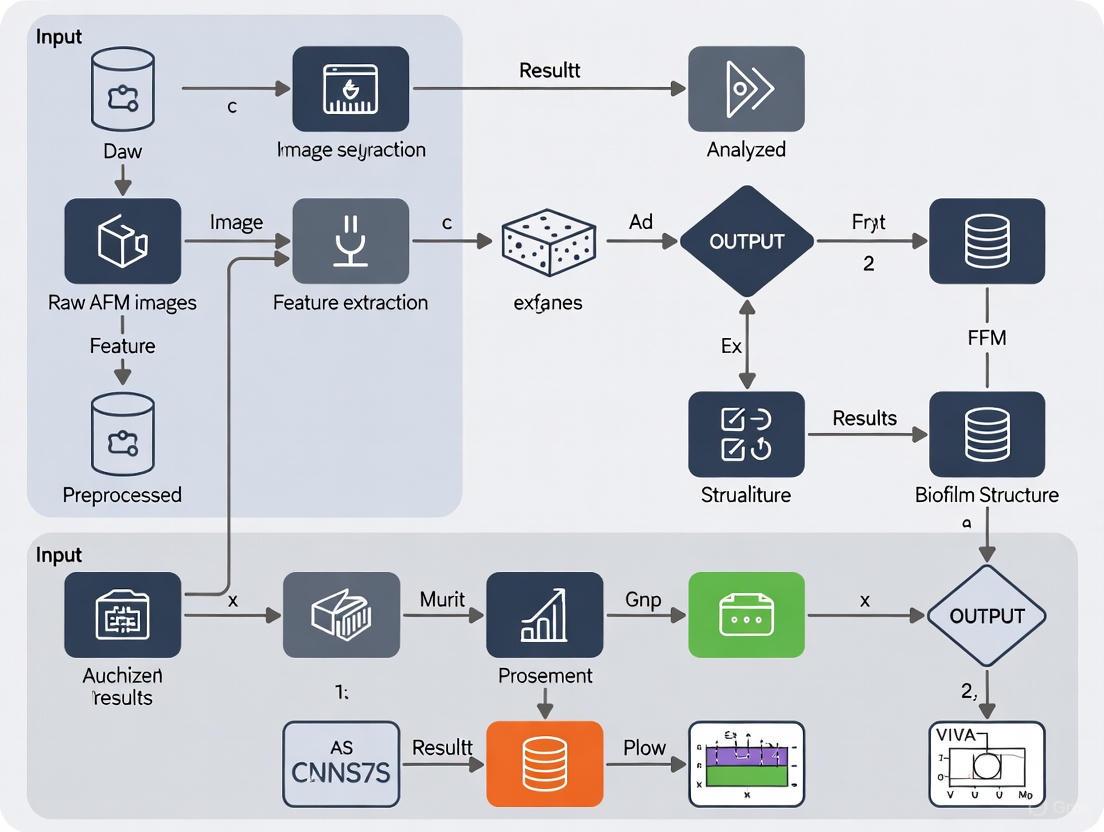
ML-Enhanced AFM Biofilm Analysis Workflow
The integration of machine learning with established experimental protocols creates a powerful pipeline for automated and insightful biofilm analysis. The diagram below illustrates this workflow from data acquisition to model-driven insight.
ML-AFM Biofilm Analysis Pipeline
This workflow highlights how ML models are trained on fused datasets. AFM provides high-resolution spatial and mechanical data, while complementary techniques like FT-IR and enzymatic assays supply chemical composition. The resulting model can then automatically quantify key characteristics like spatial heterogeneity and classify EPS components directly from AFM images.
Technical Support Center
Troubleshooting Guides
Guide 1: Addressing Common AFM Imaging Artifacts in Biofilm Samples
Problem 1: Unexpected or Repetitive Patterns in Images
- Symptoms: Structures appear duplicated; irregular shaped features repeat across the image; trenches appear smaller than expected.
- Cause: Tip artefacts, often from a broken or contaminated AFM probe [10].
- Solution: Replace the AFM probe with a new, sharp one. Ensure proper probe handling and storage to prevent contamination [10].
Problem 2: Repetitive Lines Across the Image
- Symptoms: Horizontal or vertical lines repeating at regular intervals.
- Cause A: Electrical noise, often at 50/60 Hz, from building circuits or other instrumentation [10].
- Solution: Image during quieter electrical periods (e.g., early mornings or late evenings). If possible, relocate the AFM to a location with cleaner power [10].
- Cause B: Laser interference from reflections off a highly reflective sample surface [10].
- Solution: Use an AFM probe with a reflective coating (e.g., gold or aluminum) on the cantilever to prevent spurious laser reflections [10].
Problem 3: Streaks on Images
- Symptoms: Long, directional smearing or streaks in the image.
- Cause A: Environmental noise or vibration from doors, traffic, or people moving nearby [10].
- Solution: Ensure the anti-vibration table is functional. Image during quieter times or use an acoustic enclosure. Place a "STOP AFM in progress" sign to alert others [10].
- Cause B: Loose particles or surface contamination on the sample [10].
- Solution: Optimize sample preparation protocols to minimize loosely adhered material. Ensure samples are thoroughly rinsed and dried if appropriate [10].
Guide 2: Optimizing AFM for Large-Area Biofilm Analysis
This guide is based on the methodology from the featured case study [14] [1] [15].
Problem: Difficulty Capturing Millimeter-Scale Biofilm Architecture
- Challenge: Conventional AFM has a small imaging area (<100 µm), making it impossible to link cellular-scale events to the functional macroscale organization of a biofilm [14] [1].
- Solution: Implement an automated large-area AFM approach.
- Equipment: Use a commercial AFM (e.g., DriveAFM from Nanosurf) equipped with an automated sample stage [15].
- Automation: Develop or use software for automated stage positioning and image acquisition with minimal user intervention [14] [15].
- Image Stitching: Employ algorithms that can stitch multiple high-resolution images together seamlessly, even with limited overlap to maximize speed [14] [1].
- Data Analysis: Integrate machine learning-based tools for automated image segmentation, cell detection, and classification to manage the high volume of data [14] [1].
Frequently Asked Questions (FAQs)
FAQ 1: What are the key advantages of using AFM over other microscopy techniques for biofilm research? AFM provides high-resolution topographical images and nanomechanical property maps without extensive sample preparation that can alter native structures (e.g., dehydration, metal coating) [1]. It can be operated under physiological conditions (in liquid), preserving the biofilm's native state, and allows for the visualization of fine structures like flagella and EPS matrix components [1] [15].
FAQ 2: My biofilm images are noisy. What post-processing steps can I apply? Several post-processing steps can significantly improve AFM image quality [16]:
- Leveling/Flattening: Corrects for sample tilt and unevenness caused by the scanning process.
- Noise Filtering: Apply spatial filters (e.g., low-pass filters for high-frequency noise, median filters for spike noise) or use Fourier transforms to remove unwanted noise from the image [16].
FAQ 3: How can Machine Learning (ML) assist in analyzing large-area AFM biofilm data? ML is transformative for handling the complex, high-volume data from large-area AFM [14] [1] [3]. Key applications include:
- Image Analysis: Automating the segmentation of images, detection of individual cells, and classification of biofilm features [14] [1].
- Classification: ML algorithms can be trained to classify biofilm maturity stages based on topographic characteristics, reducing observer bias and saving time [3].
- Scanning Optimization: AI can automate routine tasks like selecting scanning regions and optimizing scanning parameters, enabling continuous, multi-day experiments [1].
FAQ 4: What are the critical sample preparation steps for imaging Pantoea sp. biofilms with AFM? As described in the case study [1] [15]:
- Surface Treatment: Use PFOTS-treated glass coverslips or structured silicon substrates as the adhesion surface.
- Inoculation: Inoculate a petri dish containing the prepared coverslips with Pantoea sp. YR343 cells in a liquid growth medium.
- Incubation: Incubate for selected time points (e.g., ~30 minutes for initial attachment studies).
- Rinsing: Gently rinse the coverslip to remove unattached (planktonic) cells.
- Drying: Dry the sample before AFM imaging (Note: drying may not be necessary if using a liquid cell for in-situ imaging).
Experimental Protocols
Protocol 1: Analyzing Early-Stage Biofilm Assembly ofPantoea sp.YR343
Objective: To characterize the initial attachment, cellular orientation, and role of flagella in biofilm formation using large-area automated AFM.
Materials:
- Pantoea sp. YR343 (gram-negative, rod-shaped, motile bacterium with peritrichous flagella) [1] [15].
- PFOTS-treated glass coverslips or gradient-structured silicon substrates [14] [15].
- Liquid growth medium.
- Automated large-area AFM system [15].
Methodology:
- Sample Preparation: Prepare surfaces and inoculate with bacteria as described in FAQ #4 [1] [15].
- AFM Imaging:
- Mount the sample on the automated AFM stage.
- Program the system to acquire multiple contiguous high-resolution images over a millimeter-scale area.
- Use a scan size for individual images that balances resolution and acquisition time (e.g., 10x10 µm to 100x100 µm).
- Data Processing:
Expected Outcomes:
- Visualization of a preferred cellular orientation forming a distinctive "honeycomb" pattern [14] [15].
- High-resolution mapping of flagella interactions between cells, suggesting flagellar coordination beyond initial attachment [14] [1].
- Quantitative data on how surface topography (e.g., pillar/ridge spacing) disrupts or influences honeycomb structure formation [15].
Protocol 2: Machine Learning-Assisted Classification of Biofilm Maturity
Objective: To automate the classification of biofilm growth stages from AFM topographical data.
Materials:
- AFM image dataset of biofilms at various incubation times.
- ML classification software (e.g., open-access tools designed for AFM biofilm image classification) [3].
Methodology:
- Training Data: Establish a ground truth by having independent researchers manually classify AFM images into pre-defined maturity classes based on topographic features (e.g., substrate coverage, cell density, EPS presence) [3].
- Algorithm Training: Train a machine learning algorithm (e.g., a convolutional neural network) on the classified dataset.
- Validation: Validate the algorithm's performance by comparing its classification accuracy, recall, and "off-by-one" accuracy against the established ground truth [3].
Expected Outcomes:
- An automated tool capable of classifying biofilm maturity stages with high accuracy, reducing manual analysis time and observer bias [3].
Table 1: Key Quantitative Findings from Pantoea sp. YR343 AFM Analysis
| Parameter | Measured Value | Experimental Context | Significance |
|---|---|---|---|
| Cell Dimensions | ~2 µm length, ~1 µm diameter [1] [15] | Single surface-attached cell after ~30 min incubation. | Provides a baseline for cellular morphology and surface area (~2 µm²) [15]. |
| Flagella Height | ~20-50 nm [1] [15] | Appendages visualized around cells during early attachment. | Confirms the ability of AFM to resolve sub-cellular structures critical for motility and attachment. |
| Biofilm Architecture | Distinctive "honeycomb" pattern [14] [15] | Cell clusters formed after 6-8 hours of propagation. | Reveals a highly organized spatial structure beyond random clustering. |
| Inhibition Efficacy | 76.99% biofilm inhibition [17] | Treatment of Pantoea agglomerans with garlic extract. | Highlights a potential natural anti-biofilm agent by targeting quorum sensing (pagI/R gene) [17]. |
Table 2: Essential Research Reagent Solutions
| Reagent / Material | Function in Experiment |
|---|---|
| Pantoea sp. YR343 | A model gram-negative, biofilm-forming bacterium used to study early assembly dynamics and pattern formation [1] [15]. |
| PFOTS-treated Glass | A hydrophobic surface treatment used to promote and study bacterial adhesion and biofilm formation [14] [15]. |
| Structured Silicon Substrates | Surfaces with engineered pillar/ridge architectures to combinatorially screen how surface topography influences bacterial attachment and biofilm structure [15]. |
| TasA Protein (B. subtilis) | An amyloid-like protein essential for the structural integrity and wrinkling of dual-species biofilms with Pantoea agglomerans [18]. |
| Garlic Extract | A natural substance shown to inhibit Pantoea agglomerans biofilm formation by interfering with quorum sensing pathways [17]. |
Workflow Visualization
Automated AFM Biofilm Analysis Workflow
Building Your Analysis Pipeline: A Step-by-Step Guide to ML-Driven AFM
Frequently Asked Questions (FAQs)
Q1: What are the main advantages of using large-area, automated AFM for biofilm research? Automated large-area AFM overcomes the key limitation of conventional AFM: its small imaging area (typically <100 µm), which is restricted by piezoelectric actuator constraints [1]. This new approach enables high-resolution imaging over millimeter-scale areas, allowing researchers to link cellular and sub-cellular scale features to the functional macroscale organization of biofilms. The integration of machine learning automates image stitching and analysis, providing a comprehensive view of spatial heterogeneity that was previously obscured [1].
Q2: My AFM images appear blurry and lack fine detail, even though the system says it is in feedback. What could be causing this? This symptom is typical of "false feedback," where the system stops the probe approach before it interacts with the hard surface forces [19]. The two most common causes are:
- Surface Contamination Layer: In ambient air, a layer of contamination on the sample can trap the probe. Solution: Increase the probe-surface interaction. In vibrating (tapping) mode, decrease the setpoint value; in non-vibrating (contact) mode, increase the setpoint value [19].
- Surface/Cantilever Charge: Electrostatic forces can bend the cantilever or affect vibration amplitude. Solution: Create a conductive path between the cantilever and sample, or use a stiffer cantilever [19].
Q3: How can machine learning assist in the analysis of AFM biofilm images? Machine learning (ML) transforms AFM data analysis by automating tasks that are time-consuming and prone to human bias [1]. In biofilm research, ML algorithms can be designed to:
- Classify Biofilm Maturity: ML can automatically classify AFM images of biofilms into different stages of maturity based on topographic characteristics, achieving accuracy comparable to human observers [3].
- Segment and Identify Features: ML aids in automating image segmentation, cell detection, and classification, enabling efficient extraction of quantitative parameters like cell count, confluency, and cell shape over large areas [1].
Q4: What are some common sources of artifacts in AFM images, and how can I minimize them? Artifacts are distortions of the true topography and can arise from several sources [20]:
- The Probe: A blunt, broken, or dirty tip is a common source. It can cause features to appear larger than they are or reduce image resolution. Regularly inspect and clean your tip.
- The Scanner: Thermal drift due to slow scanning can cause inaccurate distances between features. Ensure your operating environment is thermally stable.
- Image Processing: Over-processing images during leveling or filtering can introduce artifacts. Apply minimal, necessary processing steps [16].
Troubleshooting Guides
Problem 1: Failure to Achieve a Stable Image During Large-Area Scanning
| Symptom | Possible Cause | Solution | Principle |
|---|---|---|---|
| Blurry, out-of-focus image with loss of nanoscopic detail [19]. | False feedback from a surface contamination layer. | In Tapping Mode: Decrease the amplitude setpoint. In Contact Mode: Increase the deflection setpoint [19]. | Increases tip-sample interaction force to penetrate the soft contamination layer and interact with the hard surface. |
| Image distortion and false feedback, especially with soft cantilevers [19]. | Electrostatic forces between a charged cantilever and sample. | Create a conductive path between the cantilever holder and sample. If not possible, switch to a stiffer cantilever [19]. | Dissipates electrostatic charge, reducing attractive/repulsive forces that mimic hard surface contact. |
| Poor image resolution after nanoindentation or scanning on contaminated surfaces [21]. | Dirty or contaminated probe tip. | Perform cleaning indentations on a soft, sacrificial sample (e.g., gold film). Use a large trigger threshold (e.g., 2.0 V) for multiple indents in the same location [21]. | The high force interaction can knock debris off the tip. This should only be done on a sample specifically intended for tip cleaning. |
| Streaks or bands in the image [20]. | Particles moving on the surface due to the scanning tip. | Ensure the sample is securely fixed. For dispersed particles, verify that the sample preparation (e.g., spin-coating) is adequate [20]. | Prevents the tip from pushing loose material across the surface during the scan. |
Problem 2: Poor Image Quality and Artifacts After Stitching
| Symptom | Possible Cause | Solution | Principle |
|---|---|---|---|
| Misalignment or visible seams between stitched image tiles. | Drift or lack of sufficient overlap between individual scans. | Use a large-area AFM system with automated navigation and ensure minimal (~10%) overlap between tiles. Apply ML-enhanced stitching algorithms [1]. | Corrects for small positional inaccuracies and blends images using features common to adjacent tiles. |
| Uneven background or "waviness" across the stitched image. | Improper leveling of individual tiles or the final stitched image. | Apply a plane fit or polynomial leveling routine to each tile before stitching. Perform a final, gentle flattening on the complete stitched image [16]. | Removes low-frequency scanner bow and tilt, creating a flat baseline for accurate topographic measurement. |
| High-frequency noise corrupting fine detail. | Electronic or environmental noise. | Apply post-processing noise filters. A low-pass filter removes high-frequency noise. A median filter is effective at removing shot noise without blurring edges [16]. | Attenuates signal frequencies that are higher than the resolution limit of the image. |
Problem 3: Challenges in Automated Biofilm Classification
| Symptom | Possible Cause | Solution | Principle |
|---|---|---|---|
| ML model fails to classify biofilm maturity stages accurately. | Insufficient or biased training data. | Train the model on a large and diverse dataset of AFM images that have been pre-classified by human experts into distinct topographic classes [3]. | Provides the algorithm with a robust ground truth, enabling it to learn the defining features of each class. |
| Model performance is good on training data but poor on new images. | Overfitting to the training set. | Use a simplified model architecture, increase training data, or employ data augmentation techniques. Validate the model on a completely independent test set of images [3]. | Ensures the model learns generalizable features of biofilm topography rather than memorizing the training images. |
| Inconsistent classification results between different human operators. | Subjective observer bias in defining the ground truth. | Establish a clear, written classification scheme with defined topographic characteristics for each biofilm class (e.g., based on substrate coverage, cell morphology, EPS presence) [3]. | Standardizes the classification process, improving consistency for both human observers and the ML model. |
Experimental Protocols
Protocol 1: Automated Large-Area Scanning of Bacterial Biofilms
Objective: To acquire high-resolution, stitched topographical data of a bacterial biofilm over a millimeter-scale area.
1. Sample Preparation
- Strain: Pantoea sp. YR343 (gram-negative, rod-shaped, peritrichous flagella) is used as a model biofilm-forming bacterium [1].
- Substrate: Use PFOTS-treated glass coverslips to promote adhesion [1].
- Inoculation: Place coverslips in a petri dish and inoculate with bacteria in liquid growth medium.
- Incubation: Incubate for desired time (e.g., 30 min for initial attachment; 6-8 h for cluster formation).
- Rinsing: At time points, gently rinse coverslip to remove unattached cells.
- Drying: Air-dry the sample before AFM imaging [1].
2. AFM Setup and Data Acquisition
- Instrument: A large-area AFM system with automated stage control.
- Probe Selection: A sharp silicon or silicon nitride tip is appropriate for high-resolution imaging of biological samples.
- Mapping the Area: Define a rectangular grid of tiles to cover the desired millimeter-scale area. Set a minimal overlap (~10%) between tiles [1].
- Automated Scanning: Initiate the automated sequence. The system will image each tile consecutively. Machine learning algorithms can assist in selecting scanning sites and optimizing the process [1].
3. Image Processing and Stitching
- Leveling: Apply a plane fit or polynomial flattening to each individual tile to correct for tilt and scanner bow [16].
- Stitching: Use a stitching algorithm to merge the tiles into a single, large image. ML can aid in seamless stitching even with minimal overlap [1].
Protocol 2: ML-Based Classification of Biofilm Maturity from AFM Images
Objective: To train a machine learning model to automatically classify the maturity stage of a staphylococcal biofilm based on its AFM topography [3].
1. Data Preparation (Ground Truth Labeling)
- Acquire AFM Images: Collect a large set of AFM images of biofilms grown under various conditions and for different durations.
- Define Classes: Establish a classification framework. For example, define 6 distinct classes based on topographic characteristics (e.g., isolated cells, microcolonies, EPS-dominated structures) [3].
- Human Classification: Have multiple independent experts classify each image in the dataset according to the defined framework. This set of human-classified images serves as the "ground truth" [3].
2. Model Training and Validation
- Algorithm Design: Develop or select a suitable ML algorithm (e.g., a convolutional neural network) for image classification.
- Train the Model: Input the ground-truthed images to train the model to recognize the features associated with each maturity class.
- Validate Performance: Test the trained model on a separate set of images not used during training. Compare its classifications to the human-generated ground truth. A well-designed model can achieve high off-by-one accuracy (e.g., 0.91) [3].
The Scientist's Toolkit: Research Reagent Solutions
| Essential Material | Function in the Experiment |
|---|---|
| PFOTS-Treated Glass Coverslips | A hydrophobic surface treatment that promotes bacterial adhesion and facilitates the study of early-stage biofilm assembly and surface attachment dynamics [1]. |
| Soft Gold Film Sample | A sacrificial, standardized soft sample used specifically for cleaning contaminated AFM tips. Performing high-force indentations on it can knock debris off the tip without damaging it [21]. |
| Pantoea sp. YR343 | A gram-negative, rod-shaped model bacterium with peritrichous flagella. It is well-characterized for forming biofilms on abiotic surfaces, making it ideal for studying attachment and cluster formation [1]. |
| Stiff Cantilevers | Probes with a high spring constant. They are less sensitive to electrostatic forces and are therefore recommended for use in non-vibrating (contact) mode to avoid false feedback from surface charge [19]. |
Troubleshooting Guides and FAQs
Frequently Asked Questions
Q1: My stitched AFM image shows visible seams and misalignments between individual tiles. What could be the cause and solution?
A: Visible seams often result from insufficient overlap between adjacent image tiles or drift during the lengthy acquisition process. The automated large-area AFM approach addresses this by using machine learning algorithms designed to perform seamless stitching even with minimal matching features between images [1]. To fix this:
- Increase Overlap: Ensure a minimum overlap (e.g., 10-15%) between tiles during the experimental design phase to provide the algorithm with enough data for accurate alignment.
- Leverage Advanced ML Stitching: Utilize ML-based stitching algorithms that are robust to limited features. These algorithms can identify and correlate subtle, non-unique features across tiles, creating a seamless composite image without manual intervention [1].
Q2: The ML model for segmenting individual bacterial cells is performing poorly, failing to distinguish cells from the substrate or from each other in dense clusters. How can I improve its accuracy?
A: Poor segmentation accuracy typically stems from a lack of model specificity or insufficient training data. The solution involves refining the model with high-quality, task-specific data.
- Re-train with Domain-Specific Data: Models like the Segment Anything Model (SAM) show impressive zero-shot capabilities but often underperform on specialized medical or biological images without fine-tuning [22]. Fine-tuning SAM on a curated dataset of your AFM biofilm images, even with a limited number of examples, significantly boosts its performance on your specific task [22].
- Utilize Generative Models for Data Augmentation: In ultra low-data regimes, frameworks like GenSeg can be employed. GenSeg uses generative AI and multi-level optimization to create high-fidelity synthetic image-mask pairs tailored to improve segmentation outcomes [23]. This can provide the diverse training data needed to improve model robustness without extensive manual labeling.
Q3: I am encountering strange, repeating patterns in my AFM images that do not correspond to the sample. What is this and how do I resolve it?
A: This is a classic sign of a contaminated or damaged AFM probe [10]. A blunt or dirty tip can produce artifacts where irregular shapes are duplicated across the image.
- Immediate Action: Replace the AFM probe with a new, clean one.
- Prevention: Always inspect probes before use and ensure proper handling and storage to avoid contamination. Using probes from reputable manufacturers that guarantee tip sharpness can minimize this issue [10].
Q4: My AFM image appears blurry and lacks nanoscale detail, even though the system says it is in feedback. What is happening?
A: This condition, known as "false feedback," occurs when the probe interacts with a surface contamination layer or electrostatic forces before reaching the actual sample surface [24].
- For Surface Contamination: Increase the tip-sample interaction force. In vibrating (tapping) mode, this is done by decreasing the setpoint value; in non-vibrating (contact) mode, it is done by increasing the setpoint value. This forces the probe through the contamination layer to interact with the hard surface forces of the sample [24].
- For Surface/Cantilever Charge: Create a conductive path between the cantilever and the sample. If that is not possible, use a stiffer cantilever to reduce the effects of electrostatic forces [24].
Key Experimental Protocols
Protocol 1: Automated Large-Area AFM Imaging and Stitching for Biofilm Analysis
This protocol is adapted from the large-area automated AFM approach used to study Pantoea sp. YR343 biofilms [1].
Sample Preparation:
- Grow your biofilm on an appropriate substrate (e.g., PFOTS-treated glass coverslips [1]).
- At the desired time point, gently rinse the substrate to remove unattached cells.
- Air-dry the sample before AFM imaging.
AFM Setup and Automated Scanning:
- Mount the sample in the AFM.
- Define a large, millimeter-scale area to be imaged. The software will automatically divide this area into a grid of individual tiles.
- Initiate the automated scanning routine. The system will sequentially image each tile with high resolution.
Machine Learning-Based Image Stitching:
- The acquired image tiles are processed by an ML stitching algorithm.
- This algorithm identifies features in each tile and computes the optimal transformation to align them into a single, continuous large-area image.
- The output is a seamless, high-resolution topographic map of the biofilm.
Protocol 2: Fine-Tuning the Segment Anything Model (SAM) for AFM Biofilm Segmentation
This protocol is based on empirical studies for optimal fine-tuning of foundation models for medical image segmentation [22].
Data Preparation:
- Curate a dataset of AFM biofilm images with corresponding manually annotated ground-truth segmentation masks.
- Split the data into training and validation sets.
Model Selection and Setup:
Fine-Tuning Strategy:
- Employ a parameter-efficient fine-tuning strategy that updates weights in both the encoder and decoder. This has been shown to be superior to other strategies [22].
- Train the model using the curated AFM image-mask pairs.
Validation:
- Evaluate the fine-tuned model's performance on the validation set using metrics like Dice Similarity Coefficient (DSC) to confirm improved segmentation accuracy.
Data Presentation
Table 1: Quantitative Performance of Segmentation Models in Low-Data Regimes
The following table summarizes the performance of a generative segmentation framework (GenSeg) compared to established baselines, demonstrating its utility when training data is scarce. Data is expressed as Dice Similarity Coefficient (DSC) [23].
| Segmentation Task | Imaging Modality | Baseline Model (Performance DSC) | GenSeg-Augmented Model (Performance DSC) | Absolute Performance Gain |
|---|---|---|---|---|
| Placental Vessels | Fetoscopic | DeepLab: 0.31 | GenSeg-DeepLab: 0.51 | +0.206 |
| Skin Lesions | Dermoscopy | UNet: ~0.51 | GenSeg-UNet: ~0.66 | +0.150 |
| Polyps | Colonoscopy | DeepLab: ~0.52 | GenSeg-DeepLab: ~0.63 | +0.113 |
| Breast Cancer | Ultrasound | UNet: ~0.50 | GenSeg-UNet: ~0.62 | +0.126 |
Table 2: Essential Research Reagent Solutions for Automated AFM Biofilm Analysis
This table lists key materials and computational tools used in the featured experiments and the broader field [1] [22] [23].
| Item Name | Function in the Workflow | Specific Example / Note |
|---|---|---|
| PFOTS-treated Substrate | Creates a controlled hydrophobic surface for studying bacterial adhesion and early biofilm formation patterns [1]. | Used for studying Pantoea sp. YR343 [1]. |
| Segment Anything Model (SAM) | Foundation model for image segmentation that can be fine-tuned for specific tasks like segmenting bacterial cells from AFM images [22]. | Fine-tuning with parameter-efficient methods in both encoder and decoder is recommended [22]. |
| Generative Segmentation (GenSeg) Framework | A generative AI model that creates synthetic image-mask pairs to train accurate segmentation models in ultra low-data regimes [23]. | Can improve performance by 10-20% with only 50-100 training samples [23]. |
| nnU-Net | A self-configuring framework for deep learning-based biomedical image segmentation that automatically adapts to new datasets [25]. | Forms the backbone of specialized tools like TotalSegmentator [25]. |
Workflow Visualization
Diagram: Automated AFM Image Processing with ML
The diagram below illustrates the integrated workflow of large-area AFM imaging, ML-powered stitching, and AI-driven segmentation for biofilm analysis.
Troubleshooting Guides
Common Quantification Errors and Solutions
Table 1: Troubleshooting Automated Feature Extraction
| Problem | Possible Cause | Solution |
|---|---|---|
| Inaccurate Cell Counts | - Poor image segmentation due to noise or uneven illumination.- ML model confusion between cells and debris or flagella. [26] | - Pre-process images with filters to reduce noise. [27]- Retrain ML classification model with a more diverse dataset that includes examples of flagella and debris. [26] [28] |
| Incorrect Confluency Measurement | - Inconsistent thresholding for distinguishing cells from background.- Failure to separate individual cells within dense clusters. | - Use a trainable, deep-learning-based segmentation tool (e.g., SINAP in IN Carta Software) that adapts to varying image contrast. [28]- Validate confluency results against a small, manually annotated area. |
| Faulty Orientation Data | - Tip artifacts from a contaminated or broken AFM probe, distorting cell shapes. [10]- Electrical or vibrational noise creating repetitive patterns in the image. [10] | - Inspect and replace the AFM probe with a new, clean one. [10]- Use a conductive cantilever coating to reduce laser interference and image at quieter times to minimize environmental noise. [10] |
Addressing "False Feedback" During AFM Imaging
Q: My AFM images appear blurry and lack nanoscopic detail, leading to failed feature extraction. What is happening?
A: This is a common issue known as "false feedback," where the AFM's automated tip approach stops before the probe interacts with the sample's hard surface forces. This can be caused by:
- Surface Contamination Layer: A layer of contamination in ambient air can trap the probe. Solution: Increase the probe-surface interaction force by decreasing the setpoint value in vibrating mode or increasing it in non-vibrating mode to force the probe through the layer. [29]
- Surface/Cantilever Charge: Electrostatic forces can bend the cantilever or affect vibration amplitude. Solution: Create a conductive path between the cantilever and sample, or use a stiffer cantilever to reduce the effect. [29]
Frequently Asked Questions (FAQs)
Q1: Why is automated analysis like machine learning crucial for quantifying AFM biofilm data?
A: Conventional analysis of individual cell dimensions is labor-intensive and becomes a major bottleneck when characterizing biofilms, which can contain immense numbers of cells. [26] [15] Automated techniques are essential for efficiently extracting parameters like cell count, confluency, shape, and orientation across large datasets, enabling statistically powerful analysis of the entire biofilm community. [26] [27]
Q2: What are the best practices for validating an ML model for cell detection and classification?
A: The development and validation of a robust ML model should follow a strict workflow:
- Training: Use a large set of accurately annotated images ("ground truth") to train the algorithm. [27] [28]
- Validation: Tune the model using a separate validation dataset to optimize its performance. [27]
- Testing: Evaluate the final model's performance on an independent test dataset. Key performance metrics include Precision (Positive Predictive Value) and Recall (Sensitivity), which help quantify false positives and false negatives, respectively. [27]
Q3: Our automated system struggles to segment images of 3D organoids or low-contrast samples. How can this be improved?
A: Challenges with low contrast, uneven background, and complex structures are common. A deep-learning-based segmentation tool is particularly effective here. Unlike conventional fixed-parameter methods, these tools can be trained to account for significant variability in sample appearance, ensuring accurate and reliable object detection across different experimental conditions. [28]
Experimental Protocols for Validation
Protocol: Cohesive Energy Measurement via AFM Abrasion
This method provides quantitative, nanoscale data on biofilm mechanical properties, which can be correlated with structural features. [30]
- Sample Preparation: Grow a 1-day biofilm on a suitable substrate (e.g., a membrane). Equilibrate the moist biofilm in a controlled humidity chamber (~90%) to maintain consistent water content. [30]
- Baseline Imaging: Collect a non-perturbative topographic image of a defined region (e.g., 5x5 µm) at a low applied load (~0 nN). [30]
- Abrasion Phase: Zoom into a smaller sub-region (e.g., 2.5x2.5 µm) and perform repeated raster scans at an elevated load (e.g., 40 nN) to abrade the biofilm. [30]
- Post-Abrasion Imaging: Return to a low load and capture another image of the larger region to visualize the abraded area. [30]
- Data Analysis:
- Subtract the post-abrasion image from the baseline image to determine the volume of displaced biofilm.
- Calculate the frictional energy dissipated during abrasion from the friction force data.
- The cohesive energy (nJ/µm³) is calculated as the frictional energy dissipated divided by the volume of biofilm removed. [30]
Workflow: Large-Area AFM for Multiscale Analysis
This workflow enables the link between cellular/sub-cellular features and the macroscopic organization of a biofilm. [26] [15]
The Scientist's Toolkit
Table 2: Essential Research Reagents and Materials
| Item | Function in Experiment |
|---|---|
| Pantoea sp. YR343 | A gram-negative, rod-shaped model bacterium with peritrichous flagella, used for studying early-stage biofilm assembly and cellular orientation on surfaces. [26] [15] |
| PFOTS-treated Glass | A silane-based treatment used to create a controlled hydrophobic surface for studying bacterial adhesion and the formation of specific patterns like honeycomb structures. [26] [15] |
| High-Aspect-Ratio (HAR) AFM Probes | Conical probes with a high height-to-width ratio are superior for accurately resolving steep-edged features and deep trenches in structured biofilms or engineered surfaces without side-wall artifacts. [10] |
| Metallically-Coated AFM Probes | Probes with a reflective coating (e.g., gold or aluminum) prevent laser interference issues, which is critical when imaging highly reflective samples to avoid streaks and noise in the data. [10] |
Frequently Asked Questions (FAQs)
FAQ 1: What are the most common data-related issues that cause poor model performance in biofilm classification?
The most common issues stem from the data itself and include corrupt, incomplete, or insufficient data [31]. A frequent problem is class imbalance, where the dataset is skewed towards one maturity class (e.g., too many "mature" images and not enough "early-attachment" images) [32] [31]. This can cause the model to become biased and perform poorly on the under-represented classes. Other prevalent issues are overfitting, where the model memorizes the training data too closely and fails on new images, and underfitting, where the model is too simple to capture the relevant patterns [32].
FAQ 2: My model performs well on training data but poorly on new AFM images. What is happening?
This is a classic sign of overfitting [32]. It indicates that your model has learned patterns specific to your training set that do not generalize to new data. Solutions include applying feature selection techniques (e.g., PCA, Univariate Selection) to reduce complexity, implementing cross-validation during training to ensure the model is evaluated on different data subsets, and using data augmentation to artificially increase the size and diversity of your training dataset [31].
FAQ 3: How can I assess the fairness and reliability of my biofilm classification model?
Responsible AI testing is crucial. You should perform fairness testing to ensure the model's outputs are consistent across different demographic groups if such metadata exists [32]. Techniques for bias detection and mitigation, such as reweighting or resampling data, can be applied. Furthermore, focus on model transparency using tools like SHAP or LIME to understand which features in an AFM image (e.g., specific topographic structures) are driving the classification decision [32].
FAQ 4: What should I do if my model's performance degrades after it has been deployed?
Performance degradation over time is often due to model drift, where the statistical properties of the incoming AFM image data change compared to the original training data [32]. Establishing a continuous monitoring system is essential to track performance metrics like accuracy and precision. If drift is detected, it will be necessary to retrain the model with new data that reflects the current conditions [32].
Troubleshooting Guide
Common Problems and Solutions
| Problem | Possible Causes | Recommended Solutions |
|---|---|---|
| Low Accuracy on Test Set | Overfitting, Underfitting, Unbalanced Data, Incorrect Hyperparameters [32] [31] | 1. Use cross-validation for model selection [31].2. Balance the dataset via resampling or augmentation [31].3. Perform hyperparameter tuning (e.g., grid search) [31]. |
| Poor Generalization to New AFM Scans | Model Drift, Overfitting on Training Data, Inadequate Preprocessing [32] | 1. Implement ongoing performance monitoring and retrain the model periodically [32].2. Apply consistent image preprocessing (leveling, noise filtering) to all data [16].3. Use a hold-out test set from a different experimental batch for final validation. |
| Inconsistent Results Between Users | Observer Bias in Ground Truth, Lack of Standardized Protocols [3] [33] | 1. Establish a standardized, pre-labeled ground truth dataset for all users to benchmark against [3].2. Provide clear guidelines for AFM image acquisition to minimize technical variation [33]. |
| API/Deployment Errors | Incorrect Input Format, Payload Size Issues, Authentication Failures [32] | 1. Validate input data format and size before sending to the API [32].2. Test API endpoints for authentication, rate limiting, and error handling [32]. |
Performance Benchmarking
The following table summarizes key performance metrics from a published study on ML-based classification of staphylococcal biofilms, which can serve as a benchmark for your model's performance [3].
| Model / Evaluator | Mean Accuracy | Recall | Off-by-One Accuracy |
|---|---|---|---|
| Human Observers (Ground Truth) | 0.77 ± 0.18 | Not Specified | Not Specified |
| Machine Learning Algorithm | 0.66 ± 0.06 | Comparable to Human | 0.91 ± 0.05 |
Note: The "Off-by-One Accuracy" is a particularly useful metric for ordinal classification tasks like maturity staging, as it considers a prediction correct if it is within one class of the true label [3].
Experimental Protocols
Protocol 1: Standardized AFM Image Acquisition for ML
This protocol is adapted from methods used to generate consistent, high-quality training data [33] [1].
Sample Preparation:
- Grow Staphylococcus aureus biofilms in Brain-Heart Infusion (BHI) broth, which has been found more effective than Trypticase Soy Broth for biofilm formation [33].
- For enhanced biofilm yield, use a supplement mix consisting of 222.2 mM glucose, 116.9 mM sucrose, and 1000 mM NaCl [33].
- Incubate cultures statically at 37°C for varying durations to capture different maturity stages.
AFM Imaging:
- Gently rinse the biofilm sample to remove unattached planktonic cells and air-dry before imaging [1].
- Use an automated large-area AFM system if available to capture high-resolution images over millimeter-scale areas, which helps account for spatial heterogeneity [1].
- Acquire multiple images from different locations and biological replicates for each maturity stage.
Protocol 2: Data Preprocessing and ML Model Training
Image Preprocessing:
- Leveling/Flattening: Correct for unevenness caused by the AFM scanning process using plane fitting algorithms [16].
- Noise Filtering: Apply spatial filters (e.g., low-pass or median filters) to eliminate high-frequency noise unrelated to the sample's topography [16].
- Lateral Calibration: Use reference surfaces to correct for image distortions [16].
Model Training and Evaluation:
- Feature Selection: Use algorithms like Principal Component Analysis (PCA) or Random Forest-based feature importance to reduce dimensionality and select the most informative features [31].
- Model Selection: Try different algorithms (e.g., convolutional neural networks for image data) and use a validation set for initial comparison [31].
- Cross-Validation: Implement k-fold cross-validation to obtain a robust estimate of model performance and to help prevent overfitting [31].
- Hyperparameter Tuning: Optimize model-specific parameters (e.g., learning rate, number of layers) using techniques like grid search [31].
The Scientist's Toolkit: Essential Research Reagents & Materials
| Item | Function in Experiment |
|---|---|
| Brain-Heart Infusion (BHI) Broth | A growth medium found to be more effective than Trypticase Soy Broth for maximizing in vitro biofilm formation by clinical isolates of S. aureus [33]. |
| Supplement Mix (Glucose, Sucrose, NaCl) | A solution of 222.2 mM glucose, 116.9 mM sucrose, and 1000 mM NaCl used to significantly increase biofilm biomass yield in TCP assays [33]. |
| PFOTS-treated Glass Coverslips | A surface treatment used to study the initial attachment and assembly dynamics of bacterial biofilms (e.g., for Pantoea sp.) under AFM [1]. |
| Crystal Violet Stain | A dye used in the Tissue Culture Plate (TCP) method to stain adhered biofilm biomass, which is then eluted and quantified spectrophotometrically [33]. |
| Open Access Desktop Classification Tool | A machine learning algorithm designed specifically to classify AFM images of staphylococcal biofilms into one of six maturity classes, available for researcher use [3]. |
Workflow and Troubleshooting Diagrams
Biofilm ML Classification Workflow
ML Troubleshooting Logic
Frequently Asked Questions
FAQ: My AFM images are not representative of the overall biofilm structure. How can I improve this? Conventional AFM has a limited scan range (typically <100 µm), which can miss the spatial heterogeneity of millimeter-scale biofilms [1]. To address this, implement a large-area automated AFM approach. This method automates the collection of multiple high-resolution images across millimeter-scale areas and uses machine learning-based algorithms to stitch them into a seamless, comprehensive image [1].
FAQ: How can I efficiently analyze the large datasets generated by large-area AFM? Manual analysis of large-area AFM data is impractical. Leverage machine learning-based image segmentation and analysis tools [1]. These can automate the extraction of quantitative parameters such as:
- Cell count and confluency
- Cellular morphology (e.g., length, diameter)
- Cellular orientation and spatial distribution [1]
FAQ: My machine learning model performs well on planktonic cell data but fails to predict antibiotic susceptibility in biofilms. Why? Biofilms possess distinct tolerance mechanisms that are not present in planktonic cells [34]. Conventional Antibiotic Susceptibility Tests (ASTs) and models trained on their data often fail because they do not account for the biofilm phenotype [34]. Ensure your training data comes from biofilm-specific susceptibility tests, such as the Biofilm Prevention Concentration (BPC) assay, which determines the lowest antibiotic concentration that prevents 90% of biofilm growth [34].
FAQ: What analytical techniques are best for predicting biofilm susceptibility? Multiple techniques can provide machine learning-ready data. The best choice may depend on whether you are predicting MIC (planktonic susceptibility) or BPC (biofilm susceptibility) [34].
- For MIC prediction: MALDI-TOF MS has shown high accuracy (97.83%) [34].
- For BPC prediction: Multi-excitation Raman spectroscopy has shown the best performance (80.43% accuracy) [34]. Other powerful techniques include Whole-Genome Sequencing (WGS) and Isothermal Microcalorimetry (IMC), which all demonstrate potential for predicting biofilm susceptibility [34].
FAQ: How can I validate my simulated AFM images? Use dedicated software like the BioAFMviewer to simulate AFM scanning on known protein structures from the PDB database [35]. You can then directly compare the simulated graphics with your experimental hs-AFM snapshots. This helps in interpreting resolution-limited images and confirming the orientation and conformation of your sample [35].
Experimental Protocols
Protocol 1: Large-Area AFM for Early Biofilm Assembly Analysis [1]
This protocol details the use of automated large-area AFM to study the initial stages of biofilm formation with high resolution.
- Surface Preparation: Treat glass coverslips with PFOTS to create a hydrophobic surface.
- Biofilm Growth: Inoculate a petri dish containing the treated coverslips with a liquid culture of your bacterial strain (e.g., Pantoea sp. YR343).
- Sample Harvesting: At selected time points (e.g., 30 minutes for initial attachment), remove a coverslip and gently rinse it with deionized water to remove non-adherent cells.
- Drying: Air-dry the sample before AFM imaging.
- Automated AFM Imaging:
- Mount the sample on the AFM stage.
- Use automated software to define a large, millimeter-scale scanning area.
- The system will automatically acquire multiple contiguous high-resolution images with minimal overlap.
- Image Processing:
- Use machine learning-based stitching algorithms to create a seamless composite image.
- Apply ML-based segmentation for automated cell detection, classification, and morphological analysis.
Protocol 2: Predicting Tobramycin Susceptibility in P. aeruginosa Biofilms using Machine Learning [34]
This protocol outlines a workflow for building a model to predict antibiotic susceptibility in biofilms.
- Strain Preparation: Use a collection of experimentally evolved and clinical P. aeruginosa isolates.
- Data Acquisition: For each strain, perform the following:
- Whole-Genome Sequencing (WGS): Sequence genomes and map variants against a wild-type reference.
- MALDI-TOF MS: Acquire proteomic fingerprints.
- Isothermal Microcalorimetry (IMC): Measure metabolic heat flow in the presence of tobramycin.
- Multi-Excitation Raman Spectroscopy (MX-Raman): Obtain biochemical fingerprints using multiple laser wavelengths.
- Susceptibility Testing:
- Determine the Minimal Inhibitory Concentration (MIC) using standard broth microdilution for planktonic cells.
- Determine the Biofilm Prevention Concentration (BPC) in a physiologically relevant medium (e.g., SCFM2). The BPC is the lowest antibiotic concentration that prevents ≥90% of biofilm growth.
- Machine Learning Model Training:
- Train an ordinal regression model using the data from each technique (WGS, MALDI-TOF, IMC, Raman) to predict the MIC and BPC values.
- Validate the model's performance on a held-out set of clinical isolates.
Data Presentation
Table 1: Performance of Machine Learning Models in Predicting Tobramycin Susceptibility [34]
| Analytical Technique | Data Type | MIC Prediction Accuracy (±1 dilution) | BPC Prediction Accuracy (±1 dilution) |
|---|---|---|---|
| MALDI-TOF MS | Proteomic Fingerprint | 97.83% | 73.91% |
| Multi-Excitation Raman | Biochemical Fingerprint | 89.13% | 80.43% |
| Whole-Genome Sequencing | Genomic Variants | 89.13% | 76.09% |
| Isothermal Microcalorimetry | Metabolic Activity | 89.13% | 73.91% |
Accuracy±1 refers to the percentage of samples for which the predicted MIC/BPC was correct within one 2-fold dilution step.
Table 2: Key Parameters for Simulated AFM with BioAFMviewer [35]
| Parameter | Description | Impact on Simulated Image | Recommended Starting Value |
|---|---|---|---|
| Probe Sphere Radius (R) | Radius of the spherical tip at the AFM probe's end. | Larger values smooth details, smaller values resolve finer features. | 1.0 nm |
| Cone Half-Angle (α) | Half the angle of the AFM tip's conical shaft. | Larger angles increase blurring at boundaries and cavities. | 10° |
| Scanning Grid Step Size (a) | The distance between measurement points on the X-Y plane. | Larger steps create pixelated images, smaller steps improve resolution. | 0.5 nm |
The Scientist's Toolkit
Table 3: Essential Research Reagent Solutions
| Item | Function in Research |
|---|---|
| PFOTS-treated Glass | Creates a hydrophobic surface to study bacterial attachment and early biofilm assembly on abiotic surfaces [1]. |
| Synthetic Cystic Fibrosis Medium 2 (SCFM2) | A culture medium that mimics the lung environment of CF patients, promoting P. aeruginosa biofilm growth that closely resembles in vivo conditions [34]. |
| BioAFMviewer Software | A computational platform that transforms PDB protein structures into simulated AFM images, aiding in the interpretation of experimental results [35] [36]. |
Workflow Visualization
Machine Learning Workflow for Predictive Biofilm Modeling
Large-Area AFM and ML Analysis Protocol
Overcoming Practical Hurdles: Data, Algorithms, and Model Performance
In the specialized field of machine learning for automated Atomic Force Microscopy (AFM) biofilm image analysis, data scarcity presents a significant barrier to developing robust models. Biofilm architectures are inherently heterogeneous, and acquiring sufficient high-resolution training data through labor-intensive AFM processes is challenging [1]. This technical support guide provides targeted strategies to overcome data limitations, enabling researchers to build more accurate and generalizable models for analyzing microbial communities.
Frequently Asked Questions (FAQs)
Q1: Why is data augmentation particularly critical for AFM biofilm image analysis? AFM imaging of biofilms is characterized by low throughput. Conventional AFM has a limited scan area (typically <100 µm), and the process is slow and labor-intensive, making large-scale data acquisition impractical [1]. Furthermore, biofilms exhibit significant spatial heterogeneity; a small dataset cannot capture the full structural diversity, leading to models that fail to generalize. Augmentation artificially expands the dataset, helping to mitigate overfitting and improve model robustness [37].
Q2: What are the primary classical machine learning techniques used for segmenting biofilm images? Before the widespread adoption of deep learning, several classical methods were employed for segmentation tasks. These sample-efficient techniques remain valuable when labeled data is scarce [38].
- Kernel Support Vector Machines (SVM): These are supervised, non-probabilistic binary classifiers effective for segmenting images into different regions (e.g., cell vs. background). They use kernel functions to learn non-linear decision boundaries without requiring massive datasets [38].
- Random Forests: This ensemble method builds multiple decision trees and is robust to noise, a common issue in AFM data.
- Markov Random Fields: These graph-based models are effective for incorporating spatial context into the segmentation, making them suitable for capturing the cohesive structure of biofilms [38].
Q3: How do I choose between basic and advanced augmentation techniques for my biofilm dataset? The choice depends on the complexity of your task and the size of your initial dataset. The following table summarizes the key characteristics for easy comparison.
Table 1: Comparison of Data Augmentation Techniques for AFM Biofilm Images
| Technique Category | Examples | Key Advantages | Common Challenges | Ideal Use Case |
|---|---|---|---|---|
| Basic Image Manipulations | Rotation, flipping, translation, scaling, adding noise, sharpening [37] | Simple to implement; computationally inexpensive; requires minimal expertise | May not generate truly novel features; can produce unrealistic artifacts if applied aggressively | Initial model testing; small datasets requiring minor variability |
| Deep Learning-Based (Synthetic Data) | Generative Adversarial Networks (GANs), Mixup [37] | Can generate highly realistic and complex new images; learns the underlying data distribution | Computationally intensive; requires significant data to train the generator; risk of mode collapse with GANs | Large, complex projects where capturing nuanced biofilm heterogeneity is critical |
Q4: A common problem I encounter is my model performing well on training data but poorly on new AFM scans. What augmentation strategies can help? This is a classic sign of overfitting, where the model has memorized the training data instead of learning generalizable patterns. To address this:
- Apply Varied Geometric Transformations: Use random rotations (especially important as biofilms have no preferred orientation), flips, and slight elastic deformations to teach the model rotational and reflectional invariance [37].
- Introduce Photometric Changes: Modify image intensity, contrast, and add Gaussian noise to simulate variations in AFM probe conditions, surface interactions, and scanning parameters [37]. This improves model resilience to acquisition artifacts.
- Employ Synthetic Data Generation: For highly complex and heterogeneous biofilm structures, using GANs to create synthetic training data can help the model learn a more complete representation of possible biofilm architectures [37].
Troubleshooting Guide
Problem: Segmentation model fails to accurately delineate individual bacterial cells within a dense cluster.
- Symptoms: The model merges adjacent cells into a single object or fails to detect cells with weak boundary contrast.
- Diagnosis: The training data lacks sufficient examples of cell-to-cell boundaries and overlapping cellular morphologies.
- Solution:
- Preprocessing: Apply intensity normalization (e.g., clipping to the 0.5th and 99.5th percentile and rescaling to [0,1]) to standardize contrast across your dataset [39] [40]. Use denoising filters (e.g., wavelet denoising) to improve boundary clarity without losing structural details [39].
- Targeted Augmentation: Implement augmentations that specifically simulate cell crowding and boundary variations. This includes random cropping on dense regions, elastic deformations to mimic cell shape changes, and adjusting brightness/contrast to simulate varying signal strength from the AFM probe [37].
- Algorithm Selection: If using a classical approach, try a Markov Random Field model, which is robust to noise and incorporates spatial context for boundary refinement [38]. For deep learning, a U-Net architecture, which is effective for biomedical image segmentation, can be trained with the augmented data.
Problem: Model trained on one bacterial species does not generalize to another.
- Symptoms: High accuracy on the training species (e.g., Pantoea sp.) but poor performance when applied to scans of a different species or in a multispecies biofilm.
- Diagnosis: The model has learned species-specific features (e.g., a particular cell length or flagellar pattern) rather than general "bacterial cell" features.
- Solution:
- Data Diversity: Incorporate images of multiple bacterial species into your training set, even if the data for each is limited. Augmentation is critical here to maximize the utility of each multi-species image.
- Transfer Learning: Start with a model pre-trained on a larger, more general biological image dataset. Fine-tune the final layers of this model on your (augmented) multi-species AFM dataset. This allows the model to leverage general feature detectors learned from a vast corpus of data.
- Feature Engineering (for Classical ML): For methods like SVM, focus on designing or selecting features that are invariant across species, such as texture descriptors (e.g., Local Binary Patterns) or shape-agnostic context features [38].
Experimental Protocols
Protocol 1: Standardized Preprocessing Pipeline for AFM Biofilm Images
This protocol ensures data consistency before augmentation, which is a foundational step for reproducible results [39] [40].
- Background Removal: Isolate the region of interest (ROI) from the image background. For AFM images, this often involves creating a binary mask using thresholding or morphological operations and applying it to the original image.
processed_image = original_image * binary_mask[39] [40]. - Denoising: Reduce high-frequency noise introduced during AFM scanning. Apply a wavelet-denoising filter (e.g.,
denoise_waveletfunction in Python'sskimagelibrary) or a median filter to preserve edges while smoothing noise [39]. - Intensity Normalization: Standardize the dynamic range of pixel intensities across all images in the dataset to ensure consistent model input. A common method is percentile-based rescaling:
normalized_image = (image - np.percentile(image, 0.5)) / (np.percentile(image, 99.5) - np.percentile(image, 0.5))[39] [40]. - Resampling: If images have different pixel sizes, resample them to a uniform resolution. This is crucial for deep learning models that require fixed input dimensions.
Protocol 2: Implementing a Combined Augmentation Strategy Using Keras
This protocol outlines a code-based method for implementing a diverse set of augmentations.
- Define the Augmentation Layer: Use a framework like
TensorFlow/Kerasto sequentially apply multiple transformations. - Integrate into the Training Pipeline: The augmentation model can be added directly to the front of your primary model or applied to the dataset during preprocessing.
- Visual Validation: Always visually inspect the augmented images to ensure the transformations produce biologically plausible results and have not introduced undesirable artifacts.
Workflow Visualization
The following diagram illustrates the logical workflow for building a robust analysis model, from data acquisition to model deployment, highlighting the central role of augmentation.
AFM Image Analysis Workflow
The Scientist's Toolkit: Research Reagent Solutions
Table 2: Essential Computational Tools for AFM Biofilm Image Analysis
| Tool/Reagent | Function in Analysis | Application Context |
|---|---|---|
| Python (skimage, OpenCV) | Provides libraries for implementing basic image preprocessing (denoising, normalization) and augmentation (rotations, flips). | Foundational programming environment for building custom image analysis pipelines [39]. |
| TensorFlow / PyTorch | Deep learning frameworks used for building and training complex models like CNNs and GANs for segmentation and synthetic data generation. | Essential for advanced, data-hungry deep learning approaches and implementing sophisticated augmentation layers [37]. |
| Large Area Automated AFM | An advanced AFM method capable of capturing high-resolution images over millimeter-scale areas, mitigating scarcity at the source. | Used to generate initial training data that is more representative of biofilm spatial heterogeneity [1] [8]. |
| Machine Learning (SVM, Random Forest) | Sample-efficient classical algorithms for tasks like cell classification and segmentation when labeled data is limited. | Ideal for initial proof-of-concept studies or when computational resources for deep learning are constrained [38]. |
| TorchIO | A Python library specifically designed for the loading, preprocessing, and augmentation of 3D medical images. | Can be adapted for 3D AFM data or volumetric biofilm reconstructions [39]. |
Frequently Asked Questions
What is class imbalance and why is it a critical issue in machine learning for AFM biofilm analysis? Class imbalance occurs when one class of data (the majority class) significantly outnumbers another (the minority class) in a dataset [41] [42]. In Automated Atomic Force Microscopy (AFM) biofilm analysis, this is common when trying to classify rare biofilm structures or specific cellular morphologies against a backdrop of common structures [3] [14]. This imbalance can cause a model to become biased, learning to predict only the majority class well. Since the model is rarely penalized for misclassifying the minority class, it may fail to learn its distinguishing patterns, which are often the most critical for discovery, such as identifying a rare but virulent biofilm phenotype [43] [44].
When should I consider using class weights instead of resampling my data? Class weighting is a powerful strategy when you want to use your dataset in its original form without adding or removing examples. It is particularly advantageous when you have a large dataset and the act of oversampling would consume significant memory and computational time, or when undersampling would lead to a substantial loss of information from the majority class [41] [45]. Class weights are also simple to implement, as many machine learning libraries, such as scikit-learn and TensorFlow, have built-in parameters for this purpose [42] [46].
How do I calculate appropriate class weights for my imbalanced dataset?
The most common method is to set class weights to be inversely proportional to the number of examples in each class. This "balanced" scheme can be calculated automatically by setting class_weight='balanced' in scikit-learn estimators. Manually, the weight for a class is given by the formula [42]:
weight_j = n_samples / (n_classes * n_samples_j)
where n_samples is the total number of samples, n_classes is the number of unique classes, and n_samples_j is the number of samples in class j. This gives the minority class a higher weight, forcing the model to pay more attention to it [42].
Which evaluation metrics should I avoid and which should I trust for imbalanced classification? For imbalanced datasets, you should be wary of relying solely on Accuracy and the Area Under the ROC Curve (AUROC) [44]. A model that always predicts the majority class can achieve high accuracy, which is misleading. AUROC can also provide an overly optimistic view of performance when the positive class is rare [44]. Instead, use metrics derived from the Confusion Matrix and the Precision-Recall curve [44]:
- F1 Score: The harmonic mean of precision and recall. It is a single metric that balances the two [44].
- Precision: The proportion of true positives among all predicted positives.
- Recall (Sensitivity): The proportion of actual positives that were correctly identified.
- Area Under the Precision-Recall Curve (AUPRC): More informative than AUROC for imbalanced data, as it focuses directly on the performance of the positive (minority) class [44].
- Matthews Correlation Coefficient (MCC): A balanced measure that considers all four quadrants of the confusion matrix, making it robust for imbalanced datasets [44].
Troubleshooting Guides
Problem: My model achieves high accuracy but fails to detect the minority class. Diagnosis: This is a classic symptom of a model biased by class imbalance. The model has learned that always predicting the majority class is an easy way to minimize its loss [43] [44]. Solution:
- Stop using accuracy as your primary metric. Immediately switch to the F1 score, precision, recall, or AUPRC [44].
- Implement class weights. Re-train your model using the calculated class weights to penalize misclassifications of the minority class more heavily [42] [46]. In Keras, this can be done by passing a
class_weightdictionary to themodel.fit()method [46]. - Examine the confusion matrix after re-training to verify that the number of true positives has increased and false negatives have decreased [44].
Problem: After applying class weights, the model's performance on the majority class has degraded significantly. Diagnosis: The class weights applied may be too extreme, over-penalizing errors on the minority class and causing the model to become biased in the opposite direction [42]. Solution:
- Tune the class weight values. Treat the class weight ratio as a hyperparameter. Instead of using the exact inverse frequency, experiment with less aggressive weights (e.g., the square root of the inverse frequency) to find an optimal balance [41].
- Use a weighted loss function. Manually define a loss function where you multiply the loss for each sample by its class weight. This offers finer control and can be combined with other techniques [42].
- Consider hybrid approaches. Combine class weighting with data-level methods like SMOTE (Synthetic Minority Over-sampling Technique) to generate new synthetic examples for the minority class, providing more data for the model to learn from without relying solely on weight-based penalties [45].
Problem: I am seeing repetitive noise and artifacts in my AFM images that are interfering with model training. Diagnosis: AFM imaging is susceptible to various forms of noise that can be mistakenly learned by the model as genuine features, degrading its generalizability [10]. Solution:
- Identify the noise type:
- Apply the corresponding fix:
- For electrical noise, try imaging at different times (e.g., late evenings) when electrical circuits are under less load, or use a power conditioner [10].
- For tip artifacts, replace the AFM probe with a new, clean one. Ensure your sample preparation minimizes loosely adhered material [10].
- For vibration noise, ensure the anti-vibration table is functional, use an acoustic enclosure, and place "AFM in Progress" signs to minimize human activity around the instrument [10].
Evaluation Metrics for Imbalanced Data
The table below summarizes key metrics to use and avoid when evaluating models on imbalanced datasets [44].
| Metric Name | Formula | When to Use | Key Advantage for Imbalance |
|---|---|---|---|
| F1 Score | 2 * (Precision * Recall) / (Precision + Recall) | When seeking a balance between false positives and false negatives. | Harmonic mean provides a single score that balances precision and recall. |
| AUPRC (Area Under Precision-Recall Curve) | Area under the plot of Precision vs. Recall | When the positive class (minority) is of primary interest. | More informative than AUROC when the class distribution is skewed. |
| Matthews Correlation Coefficient (MCC) | (TPTN - FPFN) / √((TP+FP)(TP+FN)(TN+FP)(TN+FN)) | For a robust, overall performance measure across both classes. | Accounts for all four confusion matrix categories and is reliable for imbalanced data. |
| Precision | TP / (TP + FP) | When the cost of false positives is high (e.g., false drug discovery leads). | Measures the model's accuracy when it predicts the positive class. |
| Recall (Sensitivity) | TP / (TP + FN) | When identifying all positive instances is critical (e.g., rare disease diagnosis). | Measures the model's ability to find all relevant positive instances. |
| Metrics to Use with Caution | |||
| Accuracy | (TP + TN) / (TP + TN + FP + FN) | Can be misleading for imbalanced data; only use with other metrics. | Skewed by the majority class; a high value can hide poor minority class performance. |
| AUROC (Area Under ROC Curve) | Area under the plot of TPR (Recall) vs. FPR | Can be overly optimistic for imbalanced data; prefer AUPRC. | The FPR can be deceptively low when the number of true negatives is very large. |
Experimental Protocol: Implementing Class Weights
This protocol details the steps for mitigating class imbalance via class weighting in a biofilm image classification task.
1. Problem Formulation & Data Preparation:
- Define the classification task, e.g., "Classification of Staphylococcal Biofilm Maturity based on AFM Topographic Features" [3].
- Load and preprocess your AFM image dataset. Extract features (e.g., topographic characteristics from AFM) and corresponding labels (e.g., the 6 maturity classes) [3].
- Split the data into training, validation, and test sets, ensuring the class imbalance ratio is preserved in each split [46].
2. Class Weight Calculation:
- Calculate the class weights from the training set only to prevent data leakage.
- Method A (Automatic): Use the
compute_class_weightfunction fromsklearn.utilswithclass_weight='balanced'[42]. - Method B (Manual): Calculate weights manually using the formula
weight_j = n_samples / (n_classes * n_samples_j)[42].
3. Model Training with Weights:
- Select an algorithm (e.g., Logistic Regression, Support Vector Machine, or Neural Network).
- Pass the calculated
class_weightdictionary to the model'sfit()method during training [42] [46]. In a neural network, this means the loss function will weight each example's contribution based on its class.
4. Evaluation and Iteration:
- Predict on the held-out validation and test sets.
- Evaluate performance using robust metrics from the table above (F1, AUPRC, MCC), not just accuracy [44].
- Analyze the confusion matrix to understand the types of errors the model is making.
- Tune the class weights and other hyperparameters based on validation set performance.
Class Weighting Implementation Workflow
The Scientist's Toolkit: Research Reagent Solutions
| Item / Technique | Function / Application in AFM Biofilm Analysis |
|---|---|
| Atomic Force Microscope (AFM) | Generates high-resolution topographic images of biofilm surfaces at the nanoscale, providing the primary data for analysis [3] [14]. |
| High-Aspect-Ratio (HAR) AFM Probes | Conical probes with a high height-to-width ratio are essential for accurately resolving deep, narrow trenches and vertical structures in heterogeneous biofilms without artifacts [10]. |
| imbalanced-learn Python Library | Provides state-of-the-art resampling algorithms (e.g., SMOTE, Tomek Links) that can be used in conjunction with class weighting to handle severe imbalance [45]. |
| Class Weight Parameter | A built-in feature in scikit-learn and Keras models that automatically adjusts the loss function to penalize misclassifications of the minority class more heavily [42] [46]. |
| Reflective Coated Probes | AFM probes with a metal coating (e.g., gold, aluminum) prevent laser interference on highly reflective samples, reducing noise in the AFM signal and leading to cleaner images for model training [10]. |
| Anti-Vibration Table / Acoustic Enclosure | Isolates the AFM from environmental noise (footsteps, doors, traffic), which is crucial for acquiring the stable, high-fidelity images needed for reliable machine learning [10]. |
FAQ: How does probe geometry directly affect my AFM biofilm images and their analysis?
The geometry of the AFM probe is a primary source of image artifacts and is critical for reproducible data, especially for machine learning (ML) analysis. The image obtained is a convolution of the tip shape and the actual sample surface [47].
- Tip Radius and Resolution: The apex radius of the tip is the real limitation of the ultimate resolution of an AFM measurement. A dull tip (large radius) will cause sharp feature edges to appear rounded and small features may not be resolved at all [47].
- Sidewall Angles and Feature Shape: The sidewall angles of the tip limit the accurate imaging of steep slopes. Any feature sidewall steeper than the tip's sidewall angles will appear to have the tip's angles in the image. This leads to the lateral broadening of high features [47].
- Trench Imaging: Narrow trenches will appear both narrower and shallower than they truly are because a large tip cannot fully enter the space to touch the bottom [47].
- Impact on ML Analysis: For ML models trained to classify biofilm images [48] or segment polymer domains [49], these tip-induced artifacts can lead to misclassification or incorrect domain size calculations if the training data was acquired with inconsistent tip geometries.
The table below summarizes common artifacts and their root causes in probe geometry.
Table 1: Common AFM Image Artifacts Caused by Probe Geometry
| Image Artifact | Description | Primary Geometric Cause |
|---|---|---|
| Lateral Broadening | High surface features appear wider than they are [47]. | Large tip radius, wide tip sidewall angles [47]. |
| Edge Rounding | Sharp edges of features appear rounded [47]. | Large tip radius of curvature [47]. |
| Inaccurate Sidewall Slopes | Steep feature sidewalls are imaged with a constant, less-steep angle [47]. | Limited tip sidewall angles [47]. |
| Shallow Trench Depths | The depth between adjacent structures appears shallower than the true value [47]. | Large tip apex preventing access to the trench bottom [47]. |
| Image Doubling | Multiplication of feature images in the scan [47]. | Broken tip with multiple apexes contacting the surface [47]. |
FAQ: What are the key scanning parameters I must standardize for reproducible biofilm nano-measurements?
Standardizing the scanning environment and parameters is essential to minimize operational variables and ensure that observed changes in the biofilm are biological, not instrumental.
- Scanning Mode: For soft, adhesive biofilms, Tapping Mode (or intermittent contact mode) is often preferred as it minimizes lateral forces that can damage the sample [48] [50]. Force Spectroscopy mode is used for measuring nanomechanical properties like cohesion [30] [51].
- Environmental Control: Imaging biofilms in their hydrated state is crucial. Measurements should be performed in liquid or controlled high-humidity environments (~90%) to prevent drying artifacts that significantly change biofilm properties [30] [50].
- Cantilever Selection: The choice of cantilever depends on the mode and sample.
- For high-resolution imaging in liquid, stiff qPlus sensors (k ≥ 1 kN/m) can be used with small amplitudes to achieve high resolution without damaging the sample [50].
- For force measurements on soft biofilms, softer cantilevers are typically used. The cited protocol for neuronal cells used a silicon nitride cantilever with a spring constant of ~0.01 N/m for binding force measurements and ~14.4 N/m for imaging and elasticity measurements [52].
- Setpoint and Feedback Gains: Use the lowest possible force setpoint to image the biofilm without deformation. Optimize feedback gains to ensure the system accurately tracks the surface without introducing noise or oscillations.
Table 2: Key Scanning Parameters to Standardize for Biofilm Analysis
| Parameter | Impact on Reproducibility | Recommendation for Biofilms |
|---|---|---|
| Operation Mode | Determines interaction force and potential sample damage [50]. | Tapping Mode for imaging; Force Spectroscopy for mechanics [30] [48]. |
| Environment | Hydration state drastically affects biofilm structure and mechanics [30]. | Image in liquid or controlled humidity (>90%) to maintain hydration [30] [50]. |
| Cantilever Stiffness | Affects sensitivity to forces and image resolution [50]. | Match to mode: stiff sensors (kN/m) for high-res imaging in liquid [50]; softer levers (0.01-50 N/m) for force spectroscopy on cells [52]. |
| Applied Load | High loads cause wear, sample deformation, and damage [30]. | Use the lowest possible load for stable imaging; typically ~0 nN for imaging, ~40 nN for controlled abrasion [30]. |
| Scan Speed | Affects data quality and tip-sample interaction time. | Optimize for feature retention; typically 0.2-0.4 Hz for biofilms [48]. |
Optimization Workflow for ML-Ready AFM Data
FAQ: How can machine learning help in maintaining consistent probe condition and image quality?
Machine learning can automate critical, subjective steps in AFM operation, reducing human error and bias, which is fundamental for generating standardized, reproducible datasets.
- Automated Image Quality Assessment: Trained Convolutional Neural Networks (CNNs) can assess the quality of an AFM image in real-time, flagging images that show signs of a dull or contaminated tip [53]. This allows researchers to intervene before collecting large amounts of unusable data.
- Probe Conditioning: ML can identify specific probe defects and automatically execute probe-conditioning protocols. For instance, a trained CNN can gauge image quality and perform a conditioning routine on the probe to restore its performance without user intervention [53].
- Early-Stage Image Evaluation: ML models can predict final image quality from just the first few scan lines, saving significant time by allowing aborted scans before completion if the probe condition is poor [53].
- Autonomous Classification: As demonstrated with staphylococcal biofilms, a deep learning algorithm can classify biofilm maturity based on AFM images with an accuracy similar to human researchers (mean accuracy of 0.66 ± 0.06 for the algorithm vs. 0.77 ± 0.18 for humans), providing a rapid and unbiased standard for analysis [48].
FAQ: What is a standardized protocol for measuring biofilm cohesive strength using AFM?
This protocol measures the cohesive energy of a biofilm by calculating the frictional energy dissipated to abrade a defined volume of material [30].
Methodology:
- Sample Preparation: Grow biofilm on a suitable substrate (e.g., polyolefin membrane). For measurement, equilibrate the hydrated biofilm in a chamber at 90% humidity to maintain consistent water content [30].
- Initial Topography: Image a 5x5 μm region of the biofilm at a low applied load (~0 nN) to obtain a non-destructive baseline height image [30].
- Abrasion Phase: Zoom into a 2.5x2.5 μm sub-region. Set an elevated load (e.g., 40 nN) and perform repeated raster scans (e.g., 4 scans) to abrade the biofilm [30].
- Post-Abrasion Topography: Return to the low load and image the original 5x5 μm area again. Subtract the post-abrasion height image from the pre-abrasion image to determine the volume of displaced biofilm [30].
- Data Analysis: The cohesive energy (γ) is calculated as the frictional energy dissipated (Efriction) divided by the volume of biofilm removed (Vremoved): γ = Efriction / Vremoved [30]. This value is typically reported in nJ/μm³.
Biofilm Cohesion Measurement Protocol
The Scientist's Toolkit: Essential Materials for Reproducible AFM Biofilm Research
Table 3: Key Research Reagents and Materials for AFM Biofilm Studies
| Item | Function/Application | Example from Literature |
|---|---|---|
| Conductive AFM Probes | Essential for electrical property modes like KPFM and C-AFM [54]. | Silicon cantilevers with metal coating for electric force microscopy [54]. |
| qPlus Sensors | High-resolution imaging in liquid with high stiffness (≥1 kN/m) [50]. | Sapphire tips on qPlus sensors for imaging lipid membranes in solution [50]. |
| Silicon Nitride Tips | Standard probes for contact mode and force spectroscopy in liquid. | V-shaped Si₃N₄ tips for cohesive energy measurements on biofilms [30]. |
| Functionalized Probes | Measuring specific molecular interactions (e.g., ligand-receptor). | Fibronectin-coated AFM probe to measure integrin binding forces on neurons [52]. |
| Liquid Cell | Enables imaging in biologically-relevant liquid environments [50]. | Custom sample holder with integrated bath for stable imaging in ~420 μl of solution [50]. |
| Humidity Controller | Maintains hydration for moist biofilms outside of liquid. | Integrated AFM chamber with ultrasonic humidifier for 90% humidity control [30]. |
| Fixative (e.g., Glutaraldehyde) | Preserves biofilm structure for AFM imaging in air. | 0.1% glutaraldehyde used to fix staphylococcal biofilms on implant discs [48]. |
In the field of Atomic Force Microscopy (AFM) biofilm research, accurately classifying complex structures is fundamental to understanding microbial behavior, pathogenicity, and response to treatments. For years, this task has relied on human expertise, a process that is both time-consuming and variable. The emergence of Machine Learning (ML) for automated image analysis presents a paradigm shift, offering the potential for high-throughput, reproducible classification. This technical support center guide is designed within the broader context of ML for automated AFM biofilm image analysis. It addresses a critical question: how does the performance of these ML models compare to human-level accuracy? The following sections provide benchmarking data, detailed experimental protocols, and troubleshooting guides to help researchers and drug development professionals navigate this evolving landscape, ensuring their classification algorithms achieve and surpass the rigorous standards required for scientific and clinical applications.
Performance Benchmarking: Human vs. Machine Learning
Multiple studies have directly compared the performance of human classifiers and machine learning models across various scientific tasks. The consolidated findings demonstrate that ML can not only match but often exceed human performance in classification accuracy and reliability.
Table 1: Benchmarking Human vs. Machine Learning Classification Performance
| Benchmarking Metric | Human Performance | Machine Learning Performance | Context & Notes |
|---|---|---|---|
| Overall Accuracy (F1 Score) | Lower than ML (exact score varies) [55] | 2-15 standard errors higher than humans [55] | Classification of scientific research abstracts to discipline groups [55]. |
| Inter-Rater Reliability (Fleiss' κ) | Lower consistency [55] | Consistently higher reliability [55] | Different human classifiers showed more variation than different ML models [55]. |
| Performance in Top Percentile | Can outperform ML in limited cases [55] | Generally outperforms the average human [55] | The top 5% of human classifiers can sometimes outperform ML, but identifying them is costly [55]. |
| Specific Theme Recall (Innovator) | Base for comparison [56] | High Recall: 0.98 [56] | Classification of open-text reports on doctor performance [56]. |
| Specific Theme Recall (Popular) | Base for comparison [56] | High Recall: 0.97 [56] | Classification of open-text reports on doctor performance [56]. |
| Specific Theme Recall (Respected) | Base for comparison [56] | High Recall: 0.87 [56] | Classification of open-text reports on doctor performance [56]. |
| Specific Theme Recall (Professional) | Base for comparison [56] | Recall: 0.82 [56] | Classification of open-text reports on doctor performance [56]. |
| Specific Theme Recall (Interpersonal) | Base for comparison [56] | Recall: 0.80 [56] | Classification of open-text reports on doctor performance [56]. |
A key study evaluating the classification of scientific abstracts for discipline groups found that on average, "ML is more accurate than human classifiers, across a variety of training and test datasets" [55]. Furthermore, ML classifiers demonstrated superior reliability, meaning that different models were more consistent in assigning the same classification to a given abstract compared to different human classifiers [55]. This suggests that ML can provide a more standardized and reproducible approach to classification tasks in research.
Experimental Protocols for Benchmarking Studies
To ensure the validity and reproducibility of your own benchmarking experiments, it is crucial to follow structured protocols. Below are detailed methodologies for both the human classification and ML training aspects, drawn from published research.
Protocol 1: Human Classification Task Design
This protocol outlines the steps for setting up a human classification task to generate ground truth data or for direct comparison with ML models.
Objective: To collect and evaluate human-generated classifications for a set of data samples (e.g., AFM biofilm images, research abstracts). Materials: Dataset for classification, participant recruitment pool, coding framework (themes/categories), data collection platform (e.g., online survey tool). Procedure:
- Dataset Preparation: Select and prepare a representative sample of data. For AFM images, this may involve pre-processing (leveling, noise filtering) to ensure consistent quality [16].
- Coder Recruitment & Screening: Recruit human classifiers with relevant expertise (e.g., postgraduate researchers for scientific abstracts). Screen for aptitude with a short example task [55].
- Framework Development: Define a clear coding framework. This can be a fixed set of discipline groups [55] or inductively developed themes (e.g., "professionalism," "interpersonal skills") [56].
- Task Execution: Conduct the classification task in a controlled environment. Provide clear instructions and the coding framework to participants.
- Data Collection & Aggregation: Collect the classifications from all participants. For analysis, you may use measures like Fleiss' κ to assess inter-rater reliability among human coders [55].
Protocol 2: Supervised Machine Learning Model Training
This protocol describes the process of training a supervised ML model for classification, using human-coded data as the ground truth.
Objective: To train a machine learning model to classify data samples into pre-defined categories based on a human-generated "ground truth" dataset. Materials: Human-coded dataset (from Protocol 1), machine learning software/library (e.g., Python scikit-learn), computational resources. Procedure:
- Data Preprocessing:
- Text Data: For text classification (e.g., abstracts, reports), create a term-document matrix. Clean the data by stemming words, removing numbers, and sparse terms (words that appear very infrequently) [56].
- Image Data: For AFM image classification, feature extraction is key. This may involve calculating morphological descriptors from the images [57] or using raw image data with deep learning.
- Feature Selection: Identify the most relevant features for the model. This could be the frequency of specific words [56] or quantitative metrics from AFM images like roughness, particle size, or mechanical properties [16] [57].
- Model Training: Split the human-coded data into training and testing sets. Train multiple ML algorithms (e.g., Support Vector Machines, ensemble methods) on the training set [55] [56].
- Model Validation: Use k-fold cross-validation (e.g., 10-fold) to robustly assess model performance and avoid overfitting [56].
- Performance Benchmarking: Evaluate the trained model on the held-out test set. Compare its performance (Accuracy, F1 Score, Recall) against the human baseline generated in Protocol 1 [55] [56].
The Scientist's Toolkit: Key Research Reagent Solutions
Table 2: Essential Materials and Tools for AFM-ML Biofilm Research
| Item / Reagent | Function / Application | Technical Notes |
|---|---|---|
| High-Aspect Ratio (HAR) Probes | To accurately resolve the topography of non-planar features like deep trenches in biofilms. | Conventional probes cannot reach the bottom of narrow trenches; HAR probes improve image resolution [10]. |
| Conical Tips | Superior for imaging vertical structures and complex biofilm architecture. | Provide better trace over surfaces with steep-edged features compared to pyramidal tips [10]. |
| Reflective Coating (Au, Al) | Coating on cantilevers to prevent laser interference from highly reflective samples. | Eliminates interference from laser light reflecting off the sample surface, reducing noise [10]. |
| Anti-Vibration Table | Isolates the AFM from environmental noise (e.g., building vibrations, traffic). | Crucial for acquiring high-resolution images; ensure the table is functioning (e.g., gas supply is not empty) [10]. |
| Term-Document Matrix | A text representation model for ML classification of open-text data (e.g., research notes). | Uses a "bag-of-words" approach, counting word frequencies for algorithm training [56]. |
| Morphological Descriptors | Quantitative features extracted from AFM images for ML model input. | Includes surface roughness, particle size/distribution, and nanomechanical properties [16] [57]. |
FAQs and Troubleshooting Guides
Frequently Asked Questions
Q1: If ML is more accurate on average, are human classifiers still needed? A1: Yes, human expertise remains critical. Humans define the classification framework, create the ground truth data for training ML models, and are essential for interpreting complex, ambiguous, or novel cases that fall outside the model's training data. The optimal approach is often human-AI teaming [58].
Q2: What is a major advantage of ML classification over human classification in large-scale studies? A2: Reliability. Different ML classifiers trained on the same data are remarkably consistent in their classifications, whereas different human classifiers often show significant variation. This makes ML superior for ensuring standardized, reproducible results across large datasets [55].
Q3: My ML model's performance has plateaued. What can I do? A3: Focus on improving your feature selection. For image analysis, this could mean extracting more sophisticated morphological descriptors or nanomechanical properties from your AFM data [16] [57]. For text data, ensure you are effectively removing sparse terms and using relevant domain-specific vocabulary.
Troubleshooting Common AFM Image Analysis Problems
Problem: Blurry or "out-of-focus" AFM images with no nanoscopic details.
- Cause 1: False Feedback from Surface Contamination. The AFM probe is interacting with a soft layer of contamination on the sample surface instead of the sample itself, tricking the system into stopping the tip approach prematurely [59].
- Solution: Increase the probe-surface interaction force. In vibrating (tapping) mode, decrease the setpoint value. This forces the probe through the contamination layer to engage the actual sample surface [59].
- Cause 2: Electrostatic Forces. Surface charge on the cantilever or sample can cause electrostatic attraction/repulsion, mimicking a true surface interaction [59].
- Solution: Create a conductive path between the cantilever and sample. If this is not possible, use a stiffer cantilever which is less susceptible to bending from electrostatic forces [59].
Problem: Unexpected, repeating patterns or duplicated structures in the image.
- Cause: Tip Artefacts. The probe tip may be broken, blunt, or contaminated [10].
- Solution: Replace the probe with a new, sharp one. A blunt tip will make features appear larger and trenches smaller than they are. Regularly inspect probes and use trusted suppliers [10].
Problem: Repetitive lines appearing across the image at a fixed frequency.
- Cause 1: Electrical Noise. Often appears as 50/60 Hz noise from building power circuits [10].
- Solution: This can be difficult to control. Try imaging during quieter periods (e.g., early morning, late evening) when electrical noise in the building is lower [10].
- Cause 2: Laser Interference. Occurs with highly reflective samples; reflected laser light interferes with the signal at the photodetector [10].
- Solution: Use a probe with a reflective coating (e.g., gold, aluminum), which helps prevent this type of interference [10].
Proving the Model: Accuracy, Clinical Correlation, and Multi-Method Validation
In the field of automated Atomic Force Microscopy (AFM) biofilm image analysis, machine learning (ML) models are tasked with classifying complex microbial structures based on topographic characteristics. Properly evaluating these models is not merely a technical exercise—it determines the reliability and scientific validity of your research findings. For researchers and drug development professionals, selecting the wrong metrics can lead to misleading conclusions about biofilm maturity, composition, and potential therapeutic efficacy.
This technical support guide provides comprehensive troubleshooting and best practices for quantifying the success of your classification models, with specific application to the challenges of AFM biofilm image analysis.
Core Metric Definitions and Interpretation
Fundamental Classification Metrics
Table 1: Core Performance Metrics for Classification Models
| Metric | Calculation | Interpretation | Biofilm Analysis Context |
|---|---|---|---|
| Accuracy | (TP+TN)/(TP+TN+FP+FN) | Overall correct classification rate | Best for balanced class distributions; less reliable with imbalanced biofilm maturity stages [60] [61] |
| Precision | TP/(TP+FP) | Proportion of positive identifications that were correct | Measures how reliable your model is when it flags a specific biofilm class [60] [61] |
| Recall (Sensitivity) | TP/(TP+FN) | Proportion of actual positives correctly identified | Critical for detecting rare but important biofilm characteristics; minimizes false negatives [60] [61] |
| F1 Score | 2×(Precision×Recall)/(Precision+Recall) | Harmonic mean of precision and recall | Balanced measure when you need to consider both false positives and false negatives [60] [61] |
| AUC-ROC | Area under ROC curve | Model's ability to distinguish between classes | Overall performance across all classification thresholds; valuable for multi-class biofilm maturity assessment [60] [61] |
Advanced and Application-Specific Metrics
Table 2: Advanced Metrics for Specialized Scenarios
| Metric | Use Case | Biofilm Research Application |
|---|---|---|
| Log Loss | Probabilistic classification models | Penalizes confident but wrong predictions; useful for calibrated probability outputs [60] [61] |
| Off-by-One Accuracy | Ordinal classification problems | Particularly relevant for biofilm maturity classes (0-5) where being off by one class is acceptable [48] |
| Confusion Matrix | Comprehensive error analysis | Visualizes specific misclassification patterns between biofilm classes [60] [62] |
Experimental Protocols for Metric Evaluation
Cross-Validation for Robust Model Assessment
Purpose: To obtain reliable performance estimates and reduce overfitting in limited AFM image datasets [60].
Methodology:
- Dataset Preparation: Divide your annotated AFM biofilm images into k subsets (folds) of approximately equal size, preserving class distribution [60]
- Iterative Training: Train your model k times, each time using k-1 folds for training and the remaining fold for validation [60]
- Performance Aggregation: Calculate the mean and standard deviation of your chosen metrics across all k iterations [60]
- Final Model Training: Train your final model on the entire dataset after determining the optimal hyperparameters [60]
Biofilm-Specific Considerations:
- Account for potential batch effects in AFM image acquisition
- Ensure representative sampling across different biofilm maturation time points
- Maintain consistent image preprocessing across all folds
Establishing Ground Truth for AFM Biofilm Images
Protocol from Staphylococcal Biofilm Classification Research [48]:
- Image Acquisition: Capture AFM images of staphylococcal biofilms on implant material discs using 5μm × 5μm scans to resolve individual bacterial cells (approximately 1.0 ± 0.5μm) [48]
- Characteristic Identification: Manually identify three key topographic characteristics: visible implant material substrate, bacterial cell coverage, and presence of extracellular matrix (ECM) [48]
- Grid-Based Annotation: Overlay a 10×10 grid on each image and calculate percentage coverage for each characteristic [48]
- Class Assignment: Assign one of six biofilm classes (0-5) based on predefined percentage thresholds for each characteristic [48]
- Inter-Observer Validation: Have multiple independent researchers classify a test set of images to establish baseline human performance and assess annotation consistency [48]
Troubleshooting Guides & FAQs
Frequently Asked Questions
Q: My model achieves 90% accuracy, but it's performing poorly in practice. What could be wrong? A: High accuracy can be misleading with imbalanced datasets. If one biofilm class dominates your dataset (e.g., mostly mature biofilms), the model may achieve high accuracy by simply predicting the majority class. Check precision and recall per class, and examine the confusion matrix for specific misclassification patterns [62] [61].
Q: How do I choose between optimizing for precision vs. recall in biofilm drug discovery? A: This depends on your research goal:
- Optimize PRECISION when false positives are costly (e.g., claiming a compound disrupts mature biofilms when it doesn't)
- Optimize RECALL when false negatives are problematic (e.g., failing to detect a hazardous biofilm formation pattern) [63] [61]
Q: What should I do when my model performs well on training data but poorly on validation data? A: This indicates overfitting. Solutions include:
- Implementing regularization techniques
- Reducing model complexity
- Increasing training data through augmentation
- Applying more stringent cross-validation [60] [64]
Q: How many AFM images do I need for reliable model evaluation? A: While dependent on complexity, research in similar domains has utilized datasets of 138+ unique AFM images with 5 images per class held out for testing. Ensure each biofilm class is sufficiently represented [48].
Common Error Patterns and Solutions
Table 3: Troubleshooting Common Metric Interpretation Problems
| Problem | Diagnosis | Solution |
|---|---|---|
| High accuracy but poor clinical relevance | Class imbalance skewing metrics | Use per-class precision/recall; employ F1 score; examine confusion matrix [62] |
| Inconsistent performance across experiments | Insufficient validation protocol | Implement k-fold cross-validation; ensure consistent data splits [60] |
| Model fails to distinguish similar biofilm classes | Inadequate feature representation | Perform error analysis to identify problematic classes; consider domain-specific augmentations [64] |
| Good ROC-AUC but poor practical performance | Inappropriate threshold selection | Adjust classification threshold based on precision-recall tradeoff specific to your application [61] |
Visualization of Model Evaluation Workflows
Model Evaluation and Error Analysis Pathway
The Scientist's Toolkit: Essential Research Reagents & Materials
Table 4: Key Experimental Materials for AFM Biofilm ML Research
| Material/Resource | Specification | Research Function |
|---|---|---|
| AFM Instrument | JPK NanoWizard IV with upright microscope | High-resolution imaging of biofilm topography and mechanical properties [48] |
| Titanium Alloy Substrates | Medical grade 5 TAN or TAV discs | Physiologically relevant surfaces for in vitro biofilm models [48] |
| Bacterial Strains | S. aureus LUH14616 | Model organism for staphylococcal biofilm formation studies [48] |
| Fixation Solution | 0.1% glutaraldehyde in MilliQ | Sample preservation for stable AFM imaging [48] |
| Annotation Framework | 6-class system based on substrate, cells, ECM | Standardized ground truth establishment for model training [48] |
| Cross-Validation Library | Scikit-learn or similar | Robust model evaluation and hyperparameter tuning [60] |
| Error Analysis Tools | ErrorAnalysis, custom visualization | Diagnosing specific model failures and improvement areas [62] |
Quantifying the success of ML classification models in AFM biofilm analysis requires careful metric selection that aligns with your research objectives. By implementing the protocols and troubleshooting approaches outlined in this guide, researchers can ensure their models provide reliable, actionable insights into biofilm characteristics and behaviors. Remember that model metrics should ultimately connect to meaningful biological outcomes—whether in understanding maturation processes, evaluating anti-biofilm compounds, or advancing therapeutic development.
Troubleshooting Guides and FAQs
Frequently Asked Questions
Q1: The accuracy of our machine learning model is significantly lower than the ~66% cited in the case study. What are the most common pitfalls during AFM image preprocessing?
- A: Low model accuracy often stems from inconsistent AFM image quality or incorrect feature extraction. Ensure your Atomic Force Microscopy (AFM) images have high resolution and minimal artifacts. The machine learning algorithm in the case study was designed to identify pre-set topographic characteristics related to the substrate, bacterial cells, and extracellular matrix [3]. Verify that your preprocessing pipeline correctly normalizes images and that the features used for training align with these defined topographic classes.
Q2: What constitutes a sufficiently large and diverse dataset for training a robust classification model?
- A: The referenced study developed and evaluated its model on a test set of staphylococcal biofilm images classified by independent researchers [3]. While an exact image count is not provided, a robust dataset should include multiple biological replicates. The journal Biofilm emphasizes that for quantitative data, the number of biological replicate samples used for imaging must be clearly reported [65]. It is recommended to use images from multiple, independent biofilm cultures to ensure the model generalizes well.
Q3: Our manual classification by different researchers shows high variability. How was inter-observer agreement quantified in the ground truth?
- A: This is a common challenge. In the foundational study, a group of independent researchers first evaluated a test set of images, achieving a mean classification accuracy of 0.77 ± 0.18 [3]. This performance benchmark established the "human-competitive" ground truth against which the machine learning algorithm's mean accuracy of 0.66 ± 0.06 was compared. The standard deviation (±0.18) explicitly quantifies the variability between human observers.
Q4: The model struggles to distinguish between adjacent maturity classes. How can this be improved?
- A: This issue is anticipated and was observed in the original research. The study reported an off-by-one accuracy of 0.91 ± 0.05 [3], meaning that over 91% of the time, the model's prediction was either correct or adjacent to the correct class. This high off-by-one accuracy suggests that the classes exist on a continuum. Instead of viewing adjacent misclassifications as complete failures, they can be treated as "near misses." Focusing on improving the model's confidence for the core characteristics of each class, rather than the boundary cases, may be a more productive strategy.
Experimental Protocols: Key Methodologies
Protocol 1: Establishing the Ground Truth with Human Observers
- Image Acquisition: Collect high-resolution AFM images of staphylococcal biofilms grown under controlled conditions [3].
- Observer Panel: Assemble a group of independent researchers trained on the 6-class classification scheme based on topographic characteristics [3].
- Blinded Classification: Provide each observer with the test set of images in a randomized order for classification.
- Data Aggregation: Compile all classifications. The mode (most frequent) classification for each image, as agreed upon by the majority of observers, is typically established as the ground truth label for that image. The mean accuracy and standard deviation across all observers and images should be calculated [3].
Protocol 2: Training and Validating the Machine Learning Algorithm
- Data Preparation: Split the dataset of AFM images (with ground truth labels) into training, validation, and test sets.
- Model Design: Develop a machine learning algorithm, such as a convolutional neural network (CNN), capable of processing image data [3].
- Model Training: Train the model on the training set, using the validation set to tune hyperparameters and prevent overfitting.
- Performance Evaluation: Evaluate the final model on the held-out test set. Report key metrics including mean accuracy, recall (sensitivity), and off-by-one accuracy, comparing them to the human observer benchmarks [3].
The following tables summarize the key performance metrics from the case study, providing a clear benchmark for your own research.
Table 1: Performance Metrics of Human Observers vs. Machine Learning Algorithm
| Metric | Human Observers | Machine Learning Algorithm |
|---|---|---|
| Mean Accuracy | 0.77 ± 0.18 [3] | 0.66 ± 0.06 [3] |
| Recall | Information Not Specified | Comparable to human performance [3] |
| Off-by-One Accuracy | Information Not Specified | 0.91 ± 0.05 [3] |
Table 2: Interpretation of Key Metrics for Model Validation
| Metric | What It Measures | Implication for Your Research |
|---|---|---|
| Mean Accuracy | The overall proportion of correct classifications. | The primary benchmark for comparing your model's performance against the case study. |
| Off-by-One Accuracy | The proportion of classifications that are either correct or one class away from the correct one. | A crucial metric for maturity classification; a high value indicates the model is largely correct on the maturity spectrum, even if not perfectly precise. |
| Recall | The model's ability to identify all relevant instances of a specific class. | Important for ensuring one maturity class is not consistently being misclassified as another. |
The Scientist's Toolkit: Research Reagent Solutions
Table 3: Essential Materials and Tools for Automated AFM Biofilm Analysis
| Item | Function/Description | Relevance to the Experiment |
|---|---|---|
| Atomic Force Microscope (AFM) | A high-resolution imaging technique that provides topographical data at the nanoscale without extensive sample preparation [1] [66]. | Primary tool for generating the biofilm images used for both manual classification and machine learning training. |
| Open Access Desktop Tool | The machine learning algorithm from the case study, made available as an open-access resource [3]. | A potential starting point or benchmark tool for researchers to classify their own AFM biofilm images. |
| Staphylococcal Strains | The microbial species used to form biofilms for the case study [3]. | Essential biological reagents for replicating the experimental system. |
| In Vitro Biofilm Model | A controlled system for growing biofilms on abiotic surfaces under defined laboratory conditions [3]. | Provides the standardized biofilm samples required for consistent imaging and analysis. |
Workflow and Model Architecture
The following diagrams illustrate the core experimental workflow and the conceptual relationship between human and machine classification, as described in the case study.
Experimental Workflow for ML Model Validation
Human vs Machine Classification Performance
Frequently Asked Questions
FAQ: My ML model is overfitting to my AFM training data and fails on new samples. How can I improve its generalizability? Overfitting often occurs when the training dataset is too small or lacks diversity, which is a common challenge in AFM due to its relatively slow imaging speed [67]. To address this:
- Increase Data Diversity: Ensure your training set includes AFM images captured using different probes and under a range of imaging conditions to account for instrumental variations [67].
- Use Robust Features: Prioritize AFM channels that provide data in absolute units (e.g., height, adhesion, deformation) over those that are instrument-specific (e.g., phase images, error signals) for better repeatability across labs [67].
- Validate Statistically: Implement simple methods to evaluate the statistical significance of your ML classification results, which is often overlooked but critical for robust findings [67].
FAQ: What is the best way to correlate ML-classified biofilm maturity stages from AFM with genomic data? The key is to establish a reliable ground truth for your AFM data that can be linked to genomic assays.
- Establish a Classification Framework: First, adopt or develop a standardized scheme to classify biofilm maturity based on topographic characteristics visible in AFM images (e.g., substrate coverage, cell morphology, extracellular matrix presence), independent of incubation time [3].
- Leverage ML for Classification: Train a machine learning algorithm to automatically classify your AFM images according to this framework. This removes observer bias and allows for high-throughput analysis of large AFM datasets [3].
- Correlate with Genomics: Once your AFM images are classified into maturity stages, you can correlate these stages with genomic data (e.g., RNA-seq) obtained from biofilms harvested at the same stages to identify stage-specific genetic signatures [68].
FAQ: Can Raman spectroscopy be integrated with our ML-AFM workflow to add biochemical information? Yes, Raman microscopy is a powerful, label-free partner technique for AFM as it provides a molecular "fingerprint" of the sample.
- Complementary Data: While AFM provides topographical and nanomechanical data, Raman spectroscopy reveals the vibrational states of molecules, offering detailed biochemical composition [69].
- Unified ML Analysis: The high-dimensional spectral data from Raman is well-suited for machine learning. Support Vector Machines (SVMs) have been successfully used to classify cell death types based on Raman spectra, and a similar approach can distinguish biofilm states or microbial species [69].
- Workflow Integration: You can perform Raman spectroscopy on the same biofilm samples to gather biochemical data. The biochemical features from Raman and the topological features from AFM can then be fused into a single ML model for a more comprehensive classification than either technique could provide alone [69] [68].
FAQ: Our automated large-area AFM scanning is generating terabytes of data. How can we manage and analyze this efficiently? Automated large-area AFM is designed to image millimeter-scale areas, which inevitably produces large, complex datasets [1].
- Automated Image Stitching: Use built-in software algorithms to seamlessly stitch together high-resolution individual scans into a single, large-area image [1].
- Implement ML-Based Analysis: Deploy machine learning tools for automated image segmentation, cell detection, and classification. This is essential for quantitatively extracting parameters like cell count, confluency, shape, and orientation from these vast datasets [1].
Troubleshooting Guides
Problem: Poor Correlation Between AFM Topography and Proteomic Assays
You find that the surface features and hardness measured by AFM do not align with the protein abundance data from your mass spectrometry analysis.
| Potential Cause | Solution | Relevant Experimental Protocol |
|---|---|---|
| Sample preparation mismatch | Ensure the biofilm samples for AFM and proteomics are prepared from the same culture batch and under identical conditions. For AFM, gently rinse to remove unattached cells but preserve the native structure [1]. | 1. Grow biofilm in triplicate.2. For AFM: Fix a sample coverslip, gently rinse with PBS, and air-dry [1].3. For Proteomics: Scrape biofilm from surface into lysis buffer for protein extraction. |
| Spatial heterogeneity | AFM measures a specific, localized area, while proteomics often uses a bulk sample. Use large-area AFM mapping to assess heterogeneity and guide a more targeted sampling for proteomics [1]. | 1. Use large-area AFM to identify and map regions of interest (e.g., dense clusters vs. sparse areas) [1].2. Use a microdissection or laser-capture technique to sample specific, mapped regions for downstream proteomic analysis. |
| ML model ignores key features | Re-evaluate the features your ML model uses for correlation. Incorporate a wider range of AFM channels (e.g., adhesion, deformation) beyond just height, as these may better reflect the underlying biochemistry [67]. | 1. From your AFM images, extract multiple physicochemical property maps (channels).2. Use feature importance analysis within your ML model to identify which AFM parameters are most predictive of your proteomic data. |
Problem: Low Accuracy in ML Classification of Biofilm AFM Images
Your machine learning algorithm performs poorly when trying to automatically classify AFM images of biofilms into different maturity stages or types.
| Potential Cause | Solution | Relevant Experimental Protocol |
|---|---|---|
| Insufficient or biased training data | Expand your training set with images representing all expected classes. Use data augmentation techniques and ensure the "ground truth" for training is validated by multiple human observers to minimize bias [3]. | 1. Establish a classification framework with 4-6 distinct classes based on AFM topography [3].2. Have multiple independent researchers classify a test set of images to establish a reliable ground truth. An accuracy of 0.77±0.18 among humans is a good benchmark [3]. |
| Non-robust AFM imaging parameters | Standardize your AFM imaging protocols. Use absolute-value channels like height and adhesion, and avoid qualitative channels like phase imaging, which are sensitive to imaging parameters and reduce model generalizability [67]. | 1. Set a standardized imaging protocol: e.g., Scan size: 10x10 µm, Resolution: 512x512 pixels, Scan rate: 0.5-1 Hz, Force setpoint: <1 nN.2. Use the same model of AFM probe for a single study to minimize probe geometry variation. |
| Incorrect ML algorithm choice | For smaller AFM image databases (a common scenario), avoid deep-learning methods that require huge datasets. Instead, use classic ML methods like decision trees, regression models, or non-deep learning neural networks [67]. | 1. For a dataset of <10,000 images, start with non-deep learning models.2. Use a random forest classifier or support vector machine (SVM). An ML model for AFM biofilm images has achieved an accuracy of 0.66±0.06 and an off-by-one accuracy of 0.91±0.05 [3]. |
The Scientist's Toolkit: Essential Research Reagents & Materials
| Item | Function in ML-AFM Biofilm Research |
|---|---|
| PFOTS-treated glass coverslips | Creates a hydrophobic surface to promote controlled and uniform bacterial attachment for consistent AFM imaging of early-stage biofilm formation [1]. |
| Pantoea sp. YR343 (or other model strain) | A well-characterized, gram-negative bacterium used as a model system for studying biofilm assembly, structure, and genetics [1]. |
| Flagella-deficient mutant strain | A genetically modified control strain used to confirm the identity of filamentous appendages (e.g., flagella) seen in high-resolution AFM images [1]. |
| Open-access ML classification tool | Software algorithms, sometimes available as open-access desktop tools, designed specifically for classifying AFM biofilm images based on pre-set topographic characteristics [3]. |
| Raman Microscope with Cell Chamber | Enables label-free, biochemical "fingerprinting" of live biofilms via Raman spectroscopy, providing complementary data to AFM for correlative ML analysis [69]. |
| Support Vector Machine (SVM) Algorithm | A powerful machine learning model particularly effective for classifying high-dimensional data, such as Raman spectra or features extracted from AFM images [69] [67]. |
Experimental Workflows & Data Correlation
The following diagrams outline the core methodologies for integrating ML-AFM with other omics technologies.
Workflow for Correlative ML-AFM and Genomics
Workflow for Integrating ML-AFM with Raman Spectroscopy
Biofilms are complex, heterogeneous microbial communities that pose significant challenges in medical, industrial, and environmental contexts. Their analysis is crucial for developing effective control strategies, but traditional methods often fail to capture the full scope of their structural complexity. Conventional Atomic Force Microscopy (AFM) provides high-resolution topographical, mechanical, and functional insights at the nanoscale but is fundamentally limited by its restricted scan range (typically <100 µm) and labor-intensive operation [1]. This limitation creates a critical scale mismatch, making it difficult to link nanoscale cellular features to the functional macroscale organization of biofilms [1]. This section outlines how the integration of Machine Learning (ML) with AFM is overcoming these historical limitations, creating a powerful tool for the comprehensive analysis of biofilm assembly.
Technical Support & Troubleshooting Hub
Frequently Asked Questions (FAQs)
Q1: What does "false feedback" mean in AFM, and how can I correct it? A: False feedback occurs when the AFM's automated tip approach algorithm stops before the probe interacts with the sample's hard surface forces, often due to a surface contamination layer or electrostatic forces. This results in blurry, out-of-focus images that lack nanoscopic detail [70].
- Solution for Contamination: Increase the probe-surface interaction force. In vibrating (tapping) mode, decrease the setpoint value; in non-vibrating (contact) mode, increase the setpoint value to force the probe through the layer [70].
- Solution for Electrostatic Forces: Create a conductive path between the cantilever and the sample. If this is not possible, use a stiffer cantilever to reduce the effects of the charge [70].
Q2: My AFM images show unexpected, repeating patterns. What is the likely cause? A: This is typically a tip artifact, indicating a broken tip or contamination on the tip. A blunt tip will cause structures to appear larger and trenches to appear smaller [10].
- Solution: Replace the AFM probe with a new, clean one. Ensuring proper sample preparation to minimize loose debris can also prevent tip contamination [10].
Q3: I observe repetitive lines across my image. Is this noise? A: Yes, this is often caused by electrical or environmental noise [10].
- Solution for Electrical Noise (50 Hz): Identify if the noise frequency correlates with the scan rate. Imaging during quieter periods (e.g., early mornings) when building electrical noise is reduced can sometimes help [10].
- Solution for Environmental Noise/Vibration: Ensure the anti-vibration table is functional. Relocate the instrument to a quieter location, such as a basement, and use signage to alert others that sensitive AFM work is in progress [10].
Q4: Why can't my AFM probe resolve deep, narrow trenches in a biofilm matrix? A: Conventional pyramidal or tetrahedral tips have low aspect ratios, meaning they cannot physically reach the bottom of high-aspect-ratio features [10].
- Solution: Use a High-Aspect-Ratio (HAR) or conical AFM probe. These tips are specifically designed to access and accurately profile deep, narrow structures [10].
Essential Research Reagent Solutions
The following table details key materials and their functions for ML-AFM biofilm research, as utilized in recent studies [1].
| Research Reagent / Material | Function in ML-AFM Biofilm Analysis |
|---|---|
| Pantoea sp. YR343 | A model gram-negative, rod-shaped bacterium with peritrichous flagella used to study early-stage biofilm assembly and structure [1]. |
| PFOTS-treated Glass | A silanized glass surface treatment used to create a controlled hydrophobic substrate for studying bacterial adhesion and biofilm formation dynamics [1]. |
| High-Aspect-Ratio (HAR) Probes | AFM cantilevers with sharp, high-aspect-ratio tips that enable high-resolution imaging of complex biofilm topography, including deep pores and trenches [10]. |
| Conical AFM Tips | Superior for imaging non-planar features compared to pyramidal tips, providing a more accurate trace over steep-edged structures common in biofilms [10]. |
| Reflective Coated Probes | Cantilevers with a gold or aluminum coating that reduce laser interference from reflective samples, minimizing optical noise in the AFM signal [10]. |
Performance Comparison: ML-AFM vs. Traditional Tools
The quantitative advantages of ML-AFM over traditional imaging techniques are evident across multiple performance metrics. The table below provides a comparative analysis of common biofilm characterization methods.
Table 1: Comparative analysis of biofilm imaging techniques. Data synthesized from [1] [71].
| Technique | Best Resolution | Key Strengths | Key Limitations for Biofilm Analysis |
|---|---|---|---|
| ML-Augmented AFM | ~1 nm (cellular & sub-cellular) | Nanoscale resolution; automated large-area (mm) mapping; quantifies mechanical properties; works in liquid. | Requires specialized instrumentation and ML expertise; can be slow for very large areas. |
| Traditional AFM | ~1 nm | Nanoscale resolution; measures mechanical properties; works in liquid. | Very small scan area (<100 µm); labor-intensive; difficult to link micro- and macro-scales [1]. |
| Confocal Laser Scanning Microscopy (CLSM) | ~200 nm (diffraction-limited) | 3D visualization of live biofilms; non-destructive; can use fluorescent probes. | Requires staining; limited resolution; can suffer from photobleaching [71]. |
| Scanning Electron Microscopy (SEM) | ~1 nm | High-resolution surface imaging. | Requires sample dehydration and metal coating, distorting native structure [1] [71]. |
| Raman Spectroscopy | N/A (chemical fingerprint) | Label-free chemical identification. | Lack of spatial resolution; fluorescence interference [1]. |
Experimental Protocol: Automated Large-Area ML-AFM of Biofilms
This protocol details the methodology for analyzing the early attachment of Pantoea sp. YR343 using a large-area, ML-augmented AFM approach, as described in the recent literature [1].
Sample Preparation
- Substrate Treatment: Prepare glass coverslips by treating them with PFOTS to create a uniform, hydrophobic surface.
- Inoculation: Inoculate a Petri dish containing the treated coverslips with Pantoea sp. YR343 cells suspended in a liquid growth medium.
- Incubation: Allow biofilm development for a designated period (e.g., 30 minutes for initial attachment studies, 6-8 hours for cluster formation).
- Rinsing and Fixation: At the selected time point, remove a coverslip and gently rinse it with a clean buffer (e.g., Sigma "Water for Molecular Biology" [72]) to remove non-adherent cells. Air-dry the sample before imaging.
Automated Large-Area AFM Imaging
- Probe Selection: Select a high-resolution, sharp AFM probe (e.g., a conical or HAR tip) suitable for resolving fine features like flagella.
- Instrument Setup: Mount the sample. Use the automated tip approach to engage the surface. Employ vibrating (tapping) mode in liquid or air to minimize sample disturbance.
- Large-Area Scanning: Program the AFM software to automatically acquire a grid of contiguous, high-resolution images (e.g., 10x10 µm each) over a millimeter-scale area of interest. The overlap between individual images is minimized to maximize acquisition speed [1].
Machine Learning Data Processing and Analysis
- Image Stitching: Apply a machine learning-based image stitching algorithm to seamlessly merge the hundreds of individual AFM scans into a single, large-area, high-resolution topographic map [1].
- Segmentation & Feature Detection: Utilize a trained ML model (e.g., based on a U-Net architecture or similar) to automatically identify, segment, and classify features within the stitched image. Key parameters to extract include:
- Cell Count: The total number of bacterial cells.
- Confluency: The percentage of surface area covered by cells.
- Cellular Morphology: Dimensions (length, diameter) and orientation of individual cells [1].
- Quantitative Analysis: Analyze the extracted data to quantify spatial heterogeneity, identify patterns (e.g., the "honeycomb" pattern of Pantoea sp. [1]), and map the distribution and interactions of appendages like flagella.
Workflow Visualization
The Machine Learning Core: Enabling a New Paradigm
The performance leap in ML-AFM is driven by specific ML functionalities that automate and enhance every stage of the AFM workflow. The core ML applications in AFM-based biofilm research can be categorized as follows [1]:
- Automated Scanning & Data Acquisition: ML algorithms optimize the scanning process itself. This includes selecting regions of interest, refining tip-sample interactions to prevent damage, and using sparse scanning approaches coupled with compressed sensing to dramatically reduce image acquisition time [1].
- Large-Area Image Reconstruction: A critical bottleneck in traditional AFM is stitching many small images into a coherent large-area map. ML-powered stitching algorithms excel at seamlessly assembling images with minimal overlap and correcting for distortions, making millimeter-scale nanoscopy feasible [1].
- Intelligent Image Analysis: This is perhaps the most significant contribution. ML models, particularly convolutional neural networks (CNNs), are trained to automatically detect, segment, and classify features in the complex AFM topography data. This allows for the unsupervised quantification of millions of cells, flagella, and other structures, extracting statistical trends and patterns that are impossible to discern manually [1].
The integration of machine learning with atomic force microscopy represents a paradigm shift in biofilm research. ML-AFM directly addresses the fundamental limitations of traditional AFM and other imaging techniques by enabling automated, high-throughput, and quantitative analysis across the relevant spatial scales—from the sub-cellular to the community level. The ability to routinely obtain millimeter-scale maps with nanoscale resolution provides an unprecedented view of biofilm heterogeneity, cellular organization, and the role of appendages in early biofilm development.
Future advancements will likely focus on increasing scanning speeds further, enhancing real-time AI-driven decision-making during experiments, and achieving even tighter integration with complementary techniques like Raman spectroscopy for correlative chemical and structural analysis [71]. As these tools become more accessible, they will undoubtedly accelerate the discovery of novel anti-biofilm strategies and deepen our fundamental understanding of microbial community dynamics.
Conclusion
The integration of Machine Learning with Atomic Force Microscopy marks a revolutionary advance in biofilm research, transitioning analysis from subjective, small-scale observations to objective, high-throughput quantification. This synthesis demonstrates that ML not only automates labor-intensive tasks but also unlocks new biological insights—from flagellar interactions guiding biofilm assembly to robust classification systems for maturity that are independent of incubation time. The validated accuracy of these models, which can rival human performance, underscores their readiness for integration into research and clinical pipelines. Future directions point toward the development of real-time, closed-loop systems for dynamic biofilm monitoring and the creation of multi-modal predictive models that combine AFM data with genomic and metabolic information. For biomedical research, this technology holds immense promise for accelerating the discovery of anti-biofilm therapeutics and personalizing treatment strategies for persistent biofilm-associated infections.
References
- 1. Analysis of biofilm assembly by large area automated AFM [https://www.nature.com/articles/s41522-025-00704-y]
- 2. Overcoming Challenges and Limitations Regarding the ... [https://www.mdpi.com/2079-6439/11/10/83]
- 3. Machine learning assisted classification of staphylococcal ... [https://www.sciencedirect.com/science/article/pii/S2590207525000310]
- 4. Evaluating large language model agents for automation of ... [https://www.nature.com/articles/s41467-025-64105-7]
- 5. CoreML model correctly predicting on MacOS but not on iOS [https://stackoverflow.com/questions/79144881/coreml-model-correctly-predicting-on-macos-but-not-on-ios]
- 6. Core ML | Apple Developer Forums [https://developer.apple.com/forums/tags/core-ml]
- 7. Core ML | Apple Developer Forums [https://developer.apple.com/forums/forums/topics/machine-learning-and-ai/machine-learning-topic-core-ml]
- 8. Analysis of biofilm assembly by large area automated AFM [https://impact.ornl.gov/en/publications/analysis-of-biofilm-assembly-by-large-area-automated-afm/]
- 9. Tips and Tricks for Frustrated AFM Users [https://www.afmworkshop.com/newsletter/frustrated-with-your-afm?srsltid=AfmBOooEN2r7YrTkp-aW8B3F1-4QkKqcE3vbeoVJrWvMynDLSbtFsISb]
- 10. 4 Common Imaging Problems (and how to fix them) - NuNano [https://www.nunano.com/blog/2020/11/23/4-common-imaging-problems-and-how-to-fix-them]
- 11. Extracellular polymeric substances, a key element in ... [https://pmc.ncbi.nlm.nih.gov/articles/PMC6604936/]
- 12. Constituent of extracellular polymeric substances (EPS ... [https://bmcmicrobiol.biomedcentral.com/articles/10.1186/s12866-025-04034-z]
- 13. The role of extracellular polymeric substances of fungal ... [https://www.nature.com/articles/s41529-022-00253-1]
- 14. Analysis of biofilm assembly by large area automated AFM [https://pubmed.ncbi.nlm.nih.gov/40341406/]
- 15. Analysis of Biofilm Assembly by Large Area... | Research Square [https://www.researchsquare.com/article/rs-5537963/v1]
- 16. AFM image analysis: a comprehensive guide [https://www.digitalsurf.com/blog/demystifying-afm-image-analysis-a-comprehensive-guide/]
- 17. Anti-biofilm ability of garlic extract on Pantoea ... [https://www.sciencedirect.com/science/article/pii/S1944398624088362]
- 18. A Dual-Species Biofilm with Emergent Mechanical and ... [https://pmc.ncbi.nlm.nih.gov/articles/PMC6707914/]
- 19. Tips and Tricks for Frustrated AFM Users [https://www.afmworkshop.com/newsletter/frustrated-with-your-afm?srsltid=AfmBOoqplYZmDqD_oNx4hRd64fXt_NOl-IrqoT03eQe9WFspt8vK85cF]
- 20. 9.2: Atomic Force Microscopy (AFM) [https://chem.libretexts.org/Bookshelves/Analytical_Chemistry/Physical_Methods_in_Chemistry_and_Nano_Science_(Barron)/09%3A_Surface_Morphology_and_Structure/9.02%3A_Atomic_Force_Microscopy_(AFM)]
- 21. Troubleshooting [https://www.nanophys.kth.se/nanolab/afm/icon/bruker-help/Content/NanoIndentation/Troubleshooting.htm]
- 22. How to build the best medical image segmentation ... [https://www.melba-journal.org/papers/2025:006.html]
- 23. Generative AI enables medical image segmentation in ultra ... [https://www.nature.com/articles/s41467-025-61754-6]
- 24. Tips and Tricks for Frustrated AFM Users [https://www.afmworkshop.com/newsletter/frustrated-with-your-afm?srsltid=AfmBOopKl7hunbtDxLOmxePbOrAnIK4YVRy7KPKr5AxBn2j8HHGcdSXE]
- 25. Best Image Segmentation Models [2025] [https://averroes.ai/blog/best-image-segmentation-models]
- 26. Analysis of biofilm assembly by large area automated AFM [https://pmc.ncbi.nlm.nih.gov/articles/PMC12062311/]
- 27. The Use of Machine Learning for Image Analysis Artificial ... [https://pmc.ncbi.nlm.nih.gov/articles/PMC10575257/]
- 28. Artificial Intelligence, Machine Learning, Deep ... [https://www.moleculardevices.com/technology/ai-machine-deep-learning-cell-image-analysis]
- 29. Tips and Tricks for Frustrated AFM Users [https://www.afmworkshop.com/newsletter/frustrated-with-your-afm?srsltid=AfmBOopXsvAriO91uZV9_d5eV1qNQD-1J31IcxtLRPUjlCxDpnQ9fhS-]
- 30. Biofilm Cohesiveness Measurement Using a Novel Atomic ... [https://pmc.ncbi.nlm.nih.gov/articles/PMC1892862/]
- 31. The Lazy Data Scientist's Guide to AI/ML Troubleshooting [https://odsc.medium.com/the-lazy-data-scientists-guide-to-ai-ml-troubleshooting-abaf20479317?source=post_internal_links---------0----------------------------]
- 32. Testing machine learning models: A QA guide ... [https://www.tothenew.com/blog/unlocking-ais-potential-essential-testing-for-machine-learning-models/]
- 33. Standardization and Classification of In vitro Biofilm ... [https://pmc.ncbi.nlm.nih.gov/articles/PMC5572203/]
- 34. Harnessing machine learning to predict antibiotic ... [https://www.nature.com/articles/s41522-025-00833-4]
- 35. BioAFMviewer: An interactive interface for simulated AFM ... [https://pmc.ncbi.nlm.nih.gov/articles/PMC7710046/]
- 36. BioAFMviewer [https://www.bioafmviewer.com/]
- 37. Medical image data augmentation: techniques, comparisons ... [https://pmc.ncbi.nlm.nih.gov/articles/PMC10027281/]
- 38. Machine Learning Techniques for Biomedical Image ... [https://pmc.ncbi.nlm.nih.gov/articles/PMC7338207/]
- 39. Medical Image Preprocessing: Key Techniques & Best Practices [https://collectiveminds.health/articles/the-ultimate-guide-to-preprocessing-medical-images-techniques-tools-and-best-practices-for-enhanced-diagnosis]
- 40. Medical Image Preprocessing - MATLAB & Simulink [https://www.mathworks.com/help/medical-imaging/ug/overview-medical-image-preprocessing.html]
- 41. Class-imbalanced datasets | Machine Learning [https://developers.google.com/machine-learning/crash-course/overfitting/imbalanced-datasets]
- 42. How to Improve Class Imbalance using Class Weights in ML? [https://www.analyticsvidhya.com/blog/2020/10/improve-class-imbalance-class-weights/]
- 43. When is unbalanced data really a problem in Machine ... [https://stats.stackexchange.com/questions/283170/when-is-unbalanced-data-really-a-problem-in-machine-learning]
- 44. Limitations in Evaluating Machine Learning Models for ... [https://pmc.ncbi.nlm.nih.gov/articles/PMC10741524/]
- 45. Class Imbalance Strategies — A Visual Guide with Code [https://medium.com/data-science/class-imbalance-strategies-a-visual-guide-with-code-8bc8fae71e1a]
- 46. Classification on imbalanced data | TensorFlow Core [https://www.tensorflow.org/tutorials/structured_data/imbalanced_data]
- 47. Effect of different tip shapes on AFM measurement [https://www.nanoandmore.com/afm-tip-shape-effects?srsltid=AfmBOorR85tOQ9gGjqVkJvnK_VDOf-ouxKcuiatqAATcg8dh8Sp74FjB]
- 48. Machine learning assisted classification of staphylococcal ... [https://pmc.ncbi.nlm.nih.gov/articles/PMC12127609/]
- 49. Machine learning for analyzing atomic force microscopy ... [https://www.sciencedirect.com/org/science/article/pii/S2635098X2400202X]
- 50. Imaging in Biologically-Relevant Environments with AFM ... [https://www.nature.com/articles/s41598-018-27608-6]
- 51. A guide for nanomechanical characterization of soft matter ... [https://www.sciencedirect.com/science/article/pii/S2666166725002151]
- 52. Atomic Force Microscopy Protocol for Measurement of ... [https://pmc.ncbi.nlm.nih.gov/articles/PMC4854888/]
- 53. Machine learning approaches for improving atomic force ... [https://www.frontiersin.org/journals/physics/articles/10.3389/fphy.2024.1347648/full]
- 54. AFM Characterization of Electrical Properties [https://www.spmtips.com/library-materials-research-electrical-properties]
- 55. Evaluating human versus machine learning performance in ... [https://pmc.ncbi.nlm.nih.gov/articles/PMC7367789/]
- 56. Supervised Machine Learning Algorithms Can Classify ... [https://www.jmir.org/2017/3/e65/]
- 57. A machine learning framework for the prediction and ... [https://www.sciencedirect.com/science/article/pii/S2667318525000133]
- 58. [2304.08733] Human and AI Perceptual Differences in ... [https://arxiv.org/abs/2304.08733]
- 59. Tips and Tricks for Frustrated AFM Users [https://www.afmworkshop.com/newsletter/frustrated-with-your-afm?srsltid=AfmBOoqbT7XeFQDFxUUXfAzxCADNcVeNLEWIhVFs22wMlyLcszaiamI2]
- 60. Measuring Success: Techniques for Evaluating ... [https://www.institutedata.com/us/blog/evaluating-classification-models-in-data-science/]
- 61. Evaluating Success in Classification Problems [https://medium.com/@can-benli/evaluating-success-in-classification-problems-cc30f78b2eb5]
- 62. Error Analysis for Machine Learning Classification Models [https://www.analyticsvidhya.com/blog/2021/08/a-quick-guide-to-error-analysis-for-machine-learning-classification-models/]
- 63. Measuring success | Machine Learning [https://developers.google.com/machine-learning/managing-ml-projects/success]
- 64. A Comprehensive Guide to Error Analysis in Machine ... [https://medium.com/mlearning-ai/a-comprehensive-guide-to-error-analysis-in-machine-learning-288e353f7c8d]
- 65. A guide to publishing in Biofilm: how to avoid a desk rejection [https://pmc.ncbi.nlm.nih.gov/articles/PMC12206335/]
- 66. Microscopy Methods for Biofilm Imaging: Focus on SEM ... [https://pmc.ncbi.nlm.nih.gov/articles/PMC7828176/]
- 67. On machine learning analysis of atomic force microscopy ... [https://pmc.ncbi.nlm.nih.gov/articles/PMC11182436/]
- 68. Progressing microbial genomics: Artificial intelligence and ... [https://www.sciencedirect.com/science/article/pii/S2666521225000559]
- 69. Machine learning with label-free Raman microscopy to ... [https://pmc.ncbi.nlm.nih.gov/articles/PMC11814076/]
- 70. Tips and Tricks for Frustrated AFM Users [https://www.afmworkshop.com/newsletter/frustrated-with-your-afm?srsltid=AfmBOopYp0joWxqGw69GRrLmrIYZ4AVcXbVzCEfgLypTh8HboPSJmQbQ]
- 71. Advances in imaging techniques for real-time microbial ... [https://www.sciencedirect.com/science/article/abs/pii/S0165993625000950]
- 72. Frequently Asked Questions about Atomic Force Microscopy [https://www.afmhelp.com/index.php?option=com_content&view=article&id=49&Itemid=55]