Microbial Community Diversity Metrics: A Comprehensive Guide for Biomedical Researchers
This article provides a systematic framework for selecting and interpreting microbial diversity metrics in biomedical research.
Microbial Community Diversity Metrics: A Comprehensive Guide for Biomedical Researchers
Abstract
This article provides a systematic framework for selecting and interpreting microbial diversity metrics in biomedical research. It covers foundational ecological concepts, practical application methodologies, common analytical challenges with solutions, and comparative validation of widely used indices. Aimed at researchers and drug development professionals, this guide synthesizes current best practices to enhance the rigor, reproducibility, and biological relevance of microbiome studies in clinical and therapeutic contexts.
Understanding the Core Concepts of Microbial Diversity Measurement
Defining Alpha, Beta, and Gamma Diversity in Microbial Ecology
In microbial ecology, understanding the structure and distribution of communities is fundamental to interpreting their function and resilience. Diversity metrics provide the tools to quantify these patterns, among which alpha, beta, and gamma diversity form a foundational framework. Coined by Robert Whittaker, these measures allow ecologists to dissect diversity across different spatial scales. Alpha diversity describes the richness and evenness of species within a specific habitat or ecosystem. Beta diversity quantifies the difference in species composition between two or more habitats. Gamma diversity represents the overall species diversity across a large landscape or region, effectively combining the alpha diversity of individual sites with the beta diversity between them. For microbiologists, these metrics are indispensable for comparing communities across different environments—from the human gut to contaminated aquifers—and for understanding how these communities respond to environmental stressors, invasions, and medical interventions.
Alpha Diversity: Within-Habitat Microbial Richness
Alpha diversity is a critical measure for summarizing the complexity of a single microbial sample. However, it is not a single metric but a concept encompassing several complementary aspects, including the number of species (richness), the distribution of their abundances (evenness), and their phylogenetic relationships [1].
Key Metrics and Categories
A comprehensive analysis of alpha diversity metrics groups them into four main categories, each capturing a different facet of diversity [1]. The table below summarizes these key metric categories and their characteristics.
Table 1: Categories and Key Features of Alpha Diversity Metrics
| Category | Representative Metrics | What It Measures | Key Biological Interpretation |
|---|---|---|---|
| Richness | Chao1, ACE, Observed ASVs | Number of unique species (or ASVs) in a sample | Estimates total species count, including unobserved ones (e.g., Chao1) [1]. |
| Dominance/Evenness | Simpson, Berger-Parker, ENSPIE | Distribution of species abundances | Measures how evenly abundant species are; high dominance = a few taxa are prevalent [1]. |
| Phylogenetic | Faith's Phylogenetic Diversity (PD) | Evolutionary history encapsulated in a community | Reflects the sum of phylogenetic branch lengths connecting all species in a sample [1]. |
| Information | Shannon, Brillouin, Pielou | Uncertainty in predicting a randomly chosen species' identity | Integrates richness and evenness; higher entropy indicates greater, more uniform diversity [1]. |
Experimental Insights and Applications
The choice of alpha diversity metric can significantly influence the interpretation of experimental data. For instance, in a study of a mixed waste-contaminated aquifer, extreme stressors like low pH and heavy metals caused an 85% reduction in taxonomic richness and an 81% reduction in phylogenetic diversity in highly contaminated wells. In contrast, the decline in functional alpha diversity was more modest (55%) and statistically insignificant, demonstrating that microbial communities can maintain functional capacity despite severe taxonomic loss [2].
Furthermore, demographic studies of the human gut microbiome reveal that alpha diversity is shaped by host factors. Research using the American Gut Project data showed that age and geographic location significantly influence microbial richness and phylogenetic diversity, while sex has a minimal impact within healthy BMI ranges [3].
Beta Diversity: Dissimilarity Between Microbial Habitats
Beta diversity measures the compositional differences between microbial communities. It is crucial for understanding how microbial landscapes change across environmental gradients, geographic distances, or different host health states.
Measurement and Drivers
Beta diversity is typically calculated as the pairwise dissimilarity between samples. Common indices include Bray-Curtis (abundance-weighted) and Jaccard (presence-absence). A key concept linked to beta diversity is the Anna Karenina Principle, which posits that stressed communities become more dissimilar from one another. This was tested in the aquifer study, where the dispersion of functional gene composition was significantly higher in highly contaminated wells, indicating a pattern of stress-induced functional divergence [2].
In contrast, a study on fungal communities in rubber trees found that beta diversity exhibited a strong geographical pattern, primarily shaped by environmental variables like leaf phosphorus and soil available potassium [4]. This highlights that the drivers of beta diversity are context-dependent and can be decoupled from the drivers of alpha diversity.
Gamma diversity represents the total species diversity observed across a large geographic region or ecosystem. It is the pool from which local communities (alpha diversity) are drawn and is influenced by the turnover between those communities (beta diversity). In the aquifer study, the taxonomic and phylogenetic gamma diversities were lower in the highly contaminated wells compared to the uncontaminated ones, reflecting a regional loss of diversity due to extreme environmental stress [2].
Comparative Analysis of Diversity Metrics
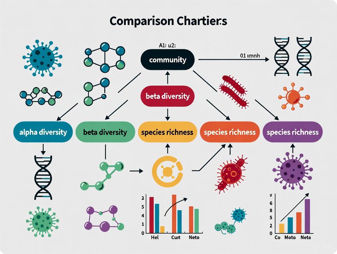
The interplay between alpha, beta, and gamma diversity provides a holistic picture of microbial systems. The following diagram illustrates their logical relationship and how they are synthesized to characterize microbial diversity across scales.
Diagram 1: Hierarchy of diversity metrics. Alpha diversity measures a single site, beta diversity links sites via turnover, and gamma diversity encompasses the entire regional species pool.
Table 2: Comparative Summary of Alpha, Beta, and Gamma Diversity in Microbial Studies
| Aspect | Alpha Diversity | Beta Diversity | Gamma Diversity |
|---|---|---|---|
| Spatial Scale | Local (within a single sample/habitat) | Between habitats or samples | Regional (across a landscape) |
| Primary Question | How diverse is this specific community? | How different are these communities from each other? | What is the total diversity of the region? |
| Key Influencing Factors | Local environmental conditions (e.g., pH, nutrients) [2], host age [3] | Geographical distance [4], environmental gradients (e.g., contamination) [2] | Historical processes, regional species pool, connectivity of habitats |
| Example Insight | Gut microbiome richness changes with host age [3]. | Contamination causes functional profiles to diverge (Anna Karenina Principle) [2]. | Regional diversity declines in heavily contaminated aquifer systems [2]. |
| Common Metrics | Chao1, Shannon, Faith's PD [1] | Bray-Curtis, Jaccard, Weighted/Unweighted UniFrac | Total species count across all sampled sites |
Essential Protocols for Diversity Analysis
Standardized protocols are vital for generating robust and comparable data in microbial ecology.
Sample Collection and DNA Sequencing
The methodology from the Mars Desert Research Station (MDRS) study provides a clear workflow for amplicon-based diversity studies [5]. Key steps include:
- Sample Collection: Swab kits (e.g., FloqSwabs) are moistened with sterile PBS to sample high-touch surfaces. For soil, samples are collected with sterile implements and stored at 4°C before transfer to -80°C for long-term storage [5].
- DNA Extraction: Use of commercial kits optimized for sample type (e.g., DNeasy PowerSoil Kit for swab pellets, DNeasy PowerMax Soil Kit for bulk soil) [5].
- Library Preparation and Sequencing: Amplification of target genetic regions (e.g., bacterial 16S rRNA V3-V4, fungal ITS1, archaeal 16S) followed by sequencing on an Illumina MiSeq platform [5].
Bioinformatics and Statistical Analysis
The QIIME 2 pipeline is the current standard for processing amplicon sequence data [5] [3]. A generalized workflow is depicted below.
Diagram 2: Standard bioinformatics workflow for microbial diversity analysis using QIIME2.
The Scientist's Toolkit: Research Reagent Solutions
Table 3: Essential Reagents and Kits for Microbial Diversity Studies
| Item | Function/Application | Example Product/Note |
|---|---|---|
| Sterile Swab Kits | Sample collection from surfaces | FloqSwabs (Copan) [5] |
| DNA Extraction Kits | Isolation of high-quality microbial genomic DNA | DNeasy PowerSoil Kit (for swabs, filters); DNeasy PowerMax Soil Kit (for bulk soil) [5] |
| PCR Primers | Amplification of taxonomic marker genes | 16S rRNA gene (V3-V4 for bacteria), ITS1 (for fungi), archaeal 16S gene [5] |
| Sequencing Platform | High-throughput sequencing of amplicons | Illumina MiSeq [5] |
| Bioinformatics Suite | Data processing, diversity calculation, and visualization | QIIME 2 pipeline [5] [3] |
| Reference Database | Taxonomic classification of sequences | GreenGenes, SILVA [3] |
Alpha, beta, and gamma diversity are interconnected metrics that provide a multi-scale lens for viewing microbial worlds. Alpha diversity quantifies local complexity, beta diversity reveals patterns of community differentiation, and gamma diversity captures the regional species pool. Contemporary research shows that these metrics can respond independently to environmental stressors [2] [4] and are influenced by distinct factors. The choice of specific alpha diversity metrics—whether richness, phylogenetic, or information-based—should be guided by the specific biological question, as each provides unique insights [1]. The standardization of protocols, from DNA extraction using specialized kits to bioinformatics processing in QIIME 2, is paramount for ensuring that findings across the field are robust, reproducible, and comparable. As microbial ecology continues to advance, this foundational framework of diversity metrics remains essential for diagnosing ecosystem health, understanding invasion dynamics [6], and guiding therapeutic developments.
In the study of microbial communities, species richness is a fundamental, yet deceptively simple, metric defined as the number of different species (or other operational taxonomic units) present in a sample [7]. However, due to constraints in sampling resources and the inherent complexity of microbial ecosystems, the observed richness in a sample—the simple count of species—almost always underestimates the true richness of the community [8]. This underestimation occurs because rare species are often missed by limited sampling efforts. To address this fundamental challenge, microbiologists and ecologists have developed statistical estimators, among which Chao1 and the Abundance-based Coverage Estimator (ACE) are two of the most widely used non-parametric methods for estimating true species richness [1] [7]. These metrics are crucial for moving beyond raw counts to more accurate estimates of microbial diversity, enabling more robust comparisons between different environments, health conditions, or therapeutic interventions. This guide provides a comparative analysis of these core richness metrics, detailing their methodologies, applications, and performance to inform research and drug development.
Comparative Analysis of Key Richness Metrics
The following table summarizes the core characteristics, mathematical foundations, and primary use cases for Observed Features, Chao1, and ACE.
Table 1: Comparison of Key Microbial Richness Metrics
| Metric | Core Concept | Key Inputs (Data) | Mathematical Formula | Primary Use Case |
|---|---|---|---|---|
| Observed Features | Simple count of distinct species/OTUs in a sample [1]. | List of species and their abundances (e.g., ASV table). | ( S_{obs} ) | Initial, intuitive assessment of sample richness; requires high/even sampling depth [7]. |
| Chao1 | Non-parametric lower bound estimator based on rare species frequency [8]. | Number of singletons (( f1 )) and doubletons (( f2 )). | ( S{obs} + \frac{f1^2}{2f2} ) (when ( f2 > 0 )) [7] | Estimating minimum richness; particularly effective for small samples and highly diverse communities [8]. |
| ACE (Abundance-based Coverage Estimator) | Non-parametric estimator that partitions data into abundant and rare species [7]. | Abundance threshold (default is 10), number of rare species (( S_{rare} )), frequencies of rare species. | ( S{abund} + \frac{S{rare}}{C{ACE}} + \frac{f1}{\hat{C}{ACE}} \hat{\gamma}{ACE}^2 ) | Estimating total richness in communities with a high proportion of rare, low-abundance species [7]. |
Beyond the core formulas, the interpretation of these metrics is guided by their relationship. Both Chao1 and ACE are highly correlated with each other and with the number of observed Amplicon Sequence Variants (ASVs) in microbiome data, suggesting that for many comparative purposes, differences in their formulas may have limited impact [1]. However, their reliability is heavily influenced by sample size and sampling effort. The performance of these estimators improves with larger sample sizes, as they converge toward the true richness [8]. Furthermore, these metrics are categorized under alpha diversity, which describes diversity within a single sample, complementing beta-diversity measures that compare diversity between samples [1].
Experimental Protocols for Metric Calculation and Validation
Standardized Data Processing Workflow
To ensure the comparability of richness metrics across different studies, a consistent data processing pipeline must be applied before calculation.
- Sequence Denoising: Process raw sequencing reads (e.g., from 16S rRNA gene sequencing) using algorithms like DADA2 or DEBLUR to resolve Amplicon Sequence Variants (ASVs). A critical consideration is that DADA2 removes all singletons as part of its denoising process, which can impact metrics like Chao1 that rely on singleton counts. Therefore, DEBLUR might be preferred for such analyses [1].
- Feature Table Construction: Build a feature table (e.g., ASV table) that records the abundance of each sequence variant in every sample.
- Rarefaction Consideration: Decide on rarefaction (subsampling to an even sequencing depth). While it can mitigate the influence of varying sequencing depths, it also discards data. Some analyses can be performed on non-rarefied data to preserve information, provided that sequencing depth has been verified to have no significant impact on key factors like the total number of ASVs and singletons [1]. All results should be validated using both approaches.
Calculation of Richness Metrics
The following workflow outlines the steps for calculating the discussed richness metrics from a processed feature table.
Figure 1: Workflow for calculating richness metrics from a processed ASV table.
Validation with Synthetic Datasets
To evaluate the statistical performance and potential biases of richness estimators, they can be applied to synthetic datasets with known properties [1].
- Method: Generate artificial microbial communities with pre-defined distributions (e.g., log-normal), total number of species, and varying levels of unevenness in species abundance (e.g., 2x, 10x, and 100x dominance ratios) [1].
- Analysis: Calculate Observed, Chao1, and ACE richness for these synthetic communities. Compare the estimates to the known true richness to assess bias, root mean square error (RMSE), and the accuracy of 95% confidence intervals [8].
- Expected Outcome: Validated estimators should significantly reduce the negative bias of observed richness and converge towards the true richness as sample size increases. A bias-corrected estimator based on the Good-Turing frequency formula has been shown to further improve upon Chao1's performance, especially in small samples or highly heterogeneous communities [8].
Applications in Research and Drug Development
Richness metrics are not merely academic exercises; they provide critical insights into host health and the efficacy of therapeutic interventions. In drug development, they can serve as surrogate endpoints—measurable markers that predict the effect of a therapy on a clinical outcome [9].
- Therapeutic Monitoring: The relationship between alpha diversity (which includes richness) and health is body-site specific. For example, increased alpha diversity in the gut is associated with a decreased risk of necrotizing enterocolitis in infants, whereas decreased alpha diversity in the vaginal community is associated with a decreased risk of bacterial vaginosis [9]. Monitoring richness can therefore help assess whether a therapy is pushing a microbiome toward a healthier state.
- Assessing Therapeutic Impact: Analysis of the historical microbiome drug development pipeline shows that drugs targeting gastrointestinal diseases, where richness is a key metric, have higher success rates transitioning from Phase 1 to Phase 2 compared to non-microbiome drugs, partly due to their favorable safety profile [10]. This underscores the value of ecological metrics in de-risking drug development.
- Unintended Consequences: The story of antibiotics provides a cautionary tale. While aimed at eradicating pathogens, broad-spectrum antibiotics cause "collateral damage" to the commensal microbiota, drastically reducing species richness and creating opportunities for hardy pathogens like Clostridium difficile to dominate [9]. This highlights the importance of monitoring richness when using therapies that perturb the microbiome.
The Scientist's Toolkit
Table 2: Essential Research Reagent Solutions for Richness Analysis
| Tool / Reagent | Function in Analysis |
|---|---|
| 16S rRNA Gene Sequencing Reagents | Provides the raw data (sequence reads) from microbial communities required for all downstream richness calculations [1]. |
| Sequence Processing Tools (QIIME 2, DADA2, DEBLUR) | Bioinformatic packages for denoising raw sequences, identifying ASVs, and constructing feature tables [1]. |
| Diversity Analysis Software (QIIME 2, R phyloseq/vegan) | Computational environments that implement the mathematical formulas for calculating Observed, Chao1, ACE, and many other diversity metrics [1]. |
| Synthetic Community Data Generators | Software scripts (e.g., in R or Python) to create simulated microbial community datasets with known properties for validating estimator performance [1]. |
Choosing the appropriate richness metric is pivotal for an accurate ecological interpretation of microbiome data. While Observed Features offers simplicity, its inherent underestimation of true diversity is a major limitation. Chao1 serves as a robust and widely adopted minimum richness estimator, particularly valuable for smaller sample sizes. ACE provides a more complex but potentially more accurate estimate for communities dominated by a high number of rare species. The choice between them depends on the specific biological question, sample size, and community characteristics. By integrating these metrics through standardized protocols and validating them with synthetic data, researchers and drug developers can generate more reliable, comparable, and insightful data, ultimately advancing our understanding of microbial ecology and its application to human health.
In the study of microbial communities, such as the gut microbiome, quantifying diversity is a fundamental step for understanding ecosystem health, stability, and its impact on the host. Diversity indices provide a way to distill complex community data into a single, comparable value. Among the most prevalent and powerful of these metrics are Shannon's Index and Simpson's Index. While both measure alpha diversity—the diversity within a single sample—they do so by weighting two key components, species richness and evenness, differently. This guide provides an objective comparison of these two indices, detailing their theoretical foundations, distinct applications, and performance in microbial research to inform the work of researchers, scientists, and drug development professionals.
Table 1: Core Comparison of Shannon's and Simpson's Indices
| Feature | Shannon's Diversity Index | Simpson's Diversity Index |
|---|---|---|
| Primary Sensitivity | More sensitive to species richness [11] [12] | More sensitive to species evenness [11] [13] |
| Mathematical Foundation | Based on information theory; measures uncertainty in predicting species identity [14]. | Based on probability; measures the chance two random individuals belong to the same species [15] [16]. |
| Common Formulas | H' = -∑(pi ln pi) Where pi is the proportion of species i [16]. |
D = ∑(pi2) Often expressed as its inverse (1/D) or compliment (1-D) for intuitive interpretation [16] [12]. |
| Value Range | Typically 0 (low diversity) to 4+ (high diversity), but can be higher [16]. | Original Index (D): 0 (infinite diversity) to 1 (no diversity).Inverse (1/D): 1 to S (number of species) [16]. |
| Interpretation of High Value | A community with high species richness and high evenness [14]. | A community with high evenness where dominant species are less likely (compliment form) [15] [16]. |
| Response to Rare Species | Gives more weight to rare species [12]. | Gives less weight to rare species [12]. |
| Primary Use Case in Microbiome | Effective for distinguishing communities with different traits, especially when rare species are of interest [17] [18]. | Assessing ecosystem stability and resilience, focusing on the dominance structure of the community [15] [13]. |
Mathematical and Conceptual Foundations
Shannon's Diversity Index
Shannon's Index (H'), derived from information theory, quantifies the uncertainty in predicting the species identity of a randomly selected individual from a sample [14]. A higher value indicates greater uncertainty and, therefore, greater diversity. The index increases with both the number of species (richness) and the equitability of their abundances (evenness). Its sensitivity to richness makes it particularly useful for detecting the presence of rare species in a community [12].
Simpson's Diversity Index
Simpson's Index (D) calculates the probability that two individuals randomly selected from a sample will belong to the same species [15] [16]. The original index, therefore, yields a higher value for less diverse communities. To make the index more intuitive, the complement (1-D) or the inverse (1/D) is often used. The Gini-Simpson index (1-D) represents the probability that two randomly selected individuals will belong to different species. Simpson's Index is more heavily influenced by the abundance of the most common species, making it a strong measure of dominance and evenness [16] [12].
Experimental Applications and Protocols in Microbiome Research
The choice between Shannon's and Simpson's indices is critical and depends on the specific research question. The following workflow outlines a typical pipeline for calculating and interpreting these indices from microbial sequencing data.
Key Experimental Findings
- Inflammatory Bowel Disease (IBD): Studies consistently show that patients with IBD have a significantly lower Shannon's Index compared to healthy controls, indicating a loss of microbial diversity and richness [14].
- Obesity and Metabolic Disorders: Research by Turnbaugh et al. found that the gut microbiome of obese individuals had a lower Shannon's Index compared to lean individuals, a finding replicated in subsequent studies [14].
- Autoimmune Diseases: A study on rheumatoid arthritis found patients had a lower Shannon's Index than healthy controls, and this diversity measure was inversely correlated with disease activity [14]. Similarly, reduced diversity has been observed in psoriatic arthritis [14].
- Comparative Performance: A framework comparing various diversity indices found that Shannon's diversity was the most effective measure for distinguishing between microbial communities with different traits within the same experiment [17].
The Scientist's Toolkit: Essential Research Reagents and Materials
The following table details key materials and tools required for conducting diversity analysis of microbial communities.
| Item | Function in Experiment |
|---|---|
| 16S rRNA Gene Sequencing | A standard method for identifying and quantifying the bacterial composition in a complex sample (e.g., gut microbiome) [17] [19]. |
| Bioinformatic Pipelines (e.g., Kraken2, Bracken) | Tools for assigning taxonomic labels to sequencing reads and estimating species abundance, which generates the input data for diversity calculations [19]. |
| Diversity Analysis Software (e.g., QIIME 2, mothur, Galaxy) | Platforms that contain built-in functions for calculating a wide array of alpha diversity indices, including Shannon and Simpson [19]. |
| Shannon's Diversity Index Formula | The mathematical metric applied to species abundance data to calculate a value representing community richness and evenness [16]. |
| Simpson's Diversity Index Formula | The mathematical metric applied to species abundance data to calculate a value representing community dominance and evenness [16]. |
Both Shannon's and Simpson's indices are indispensable tools for quantifying microbial diversity, yet they provide complementary insights. Shannon's Index is the more sensitive measure for detecting changes in species richness, particularly the presence of rare species, and has been shown to be highly effective in distinguishing between microbial communities in health and disease states. Simpson's Index provides a robust measure of community evenness and dominance, reflecting the probability of species encounters. The choice between them should be guided by the research focus: studies interested in rare taxa and overall community structure may prioritize Shannon's Index, while those focused on dominance and stability may find Simpson's Index more informative. For a comprehensive analysis, reporting both indices is often the best practice.
In microbial ecology and comparative genomics, accurately measuring biodiversity is crucial for understanding community assembly, ecosystem function, and host-microbe interactions. While traditional metrics like species richness quantify the number of taxa present, they ignore evolutionary relationships between organisms. Phylogenetic diversity metrics address this limitation by incorporating evolutionary history into diversity assessments. Among these, Faith's Phylogenetic Diversity (Faith's PD) stands as a foundational metric that quantifies the total branch length of a phylogenetic tree encompassing all species present in a community [1]. Unlike simpler richness measures, Faith's PD captures the evolutionary distinctiveness of community members, providing valuable insights into functional potential and evolutionary history preserved within ecosystems.
The growing importance of Faith's PD coincides with increased recognition that microbial communities with similar taxonomic composition may harbor significant functional differences based on phylogenetic relationships. This metric has proven particularly valuable in detecting subtle diversity patterns in host-associated microbiota [20], environmental gradients [21], and responses to anthropogenic disturbances [22]. As researchers increasingly work with large datasets containing millions of sequences, computational innovations like Stacked Faith's Phylogenetic Diversity (SFPhD) have enabled application of this powerful metric at unprecedented scales [23].
Faith's PD: Core Principles and Calculation
Conceptual Foundation and Mathematical Definition
Faith's PD measures the sum of the branch lengths of the phylogenetic tree connecting all species in a target community to their common ancestor [1]. Mathematically, for a given tree ( T ), Faith's PD for sample ( i ) is defined as:
[ PDi = \sum{j \in T} I{ij} \times \text{branchLen}j(T) ]
Where ( I{ij} ) indicates whether sample ( i ) has any features that descend from node ( j ), and ( \text{branchLen}j(T) ) represents the length of the branch leading to node ( j ) in tree ( T ) [23]. This calculation encompasses all branches connecting the root to the tips representing taxa present in the sample, effectively quantifying the total evolutionary history contained within that community.
The phylogenetic aspect of Faith's PD provides increased statistical power for detecting diversity differences between groups compared to non-phylogenetic metrics [23]. This enhanced sensitivity stems from its ability to capture evolutionarily meaningful patterns that may be obscured when treating all taxa as equally related.
Computational Implementation and Advances
Traditional computation of Faith's PD faced scalability challenges with large contemporary datasets. The reference implementation in scikit-bio used a dense matrix representation that became computationally prohibitive with trees containing millions of tips [23]. SFPhD introduced key algorithmic improvements that dramatically enhanced computational efficiency:
- Sparse matrix representation that only retains information about positions with nonzero values
- Partial aggregation of metric constituents during tree traversal, reducing memory requirements
- Balanced-parentheses vector for efficient tree topology representation
- Postorder traversal that frees memory for child nodes after processing [23]
These innovations reduced expected space complexity from O(nk) to O(n log[k]), where n is the number of samples and k is the number of vertices in the tree [23]. This enables analysis of massive datasets, such as one benchmarked study incorporating 307,237 microbiome samples with 1,264,796 phylogenetic tree tips [23].
Table 1: Key Features of Faith's Phylogenetic Diversity
| Feature | Description | Biological Interpretation |
|---|---|---|
| Evolutionary Scope | Sum of branch lengths connecting all species in a community | Total evolutionary history represented in a sample |
| Data Requirements | Phylogenetic tree with branch lengths; presence/absence or abundance data | Requires representative reference tree for placed sequences |
| Sensitivity | More sensitive than non-phylogenetic metrics for detecting group differences | Can identify subtle diversity patterns with biological significance |
| Scale Independence | Must be interpreted relative to tree scale | Values comparable only within same phylogenetic framework |
| Computational Demand | High for large trees, mitigated by SFPhD algorithm | Implementation choice affects feasible analysis scale |
Comparative Analysis of Diversity Metrics
Classification of Alpha Diversity Metrics
Microbial alpha diversity metrics can be categorized into four distinct classes based on their mathematical foundations and the aspects of diversity they emphasize [1]:
Richness metrics (Chao1, ACE, Fisher, Margalef, Menhinick, Observed, Robbins): Focus primarily on the number of unique taxa, with some incorporating correction factors for unobserved species.
Dominance/Evenness metrics (Berger-Parker, Dominance, Simpson, ENSPIE, Gini, McIntosh, Strong): Quantify the distribution of abundances among taxa, highlighting whether communities are dominated by few species or have more equitable abundance distributions.
Phylogenetic metrics (Faith's PD): Incorporate evolutionary relationships between taxa, measuring the breadth of evolutionary history represented in a community.
Information metrics (Shannon, Brillouin, Heip, Pielou): Derived from information theory, these metrics combine richness and evenness components into single values.
Each category captures different facets of microbial diversity, with Faith's PD uniquely positioned as the primary metric incorporating phylogenetic relatedness without direct dependence on abundance distributions [1].
Experimental Evidence of Faith's PD Advantages
Controlled studies across diverse host systems have demonstrated the unique value of Faith's PD in detecting biologically meaningful patterns. In a comprehensive assessment of 24 animal species from four groups (Peromyscus deer mice, Drosophila flies, mosquitoes, and Nasonia wasps) reared under controlled conditions, Faith's PD revealed significant phylosymbiosis - where ecological relatedness of host-associated microbial communities parallels host phylogeny [20]. This pattern persisted across wide-ranging evolutionary timescales, from recent speciation events (~1 million years ago) to more distantly related host genera (~108 million years ago) [20].
Transplant experiments provided functional validation for these patterns. When interspecific microbiota transplants were conducted between host species, recipients experienced survival and performance reductions, with the magnitude of fitness costs correlating with the degree of host phylogenetic divergence [20]. This demonstrates that Faith's PD captures evolutionarily informed host-microbiota relationships with direct functional consequences.
In human microbiome studies, Faith's PD has shown increased power for detecting diversity differences between demographic groups. Analysis of the FINRISK study's metagenomic data revealed that Faith's PD more effectively distinguished younger and older populations compared to non-phylogenetic metrics [23]. This enhanced sensitivity makes it particularly valuable for clinical studies seeking to identify subtle microbiome alterations associated with health status.
Table 2: Comparison of Major Alpha Diversity Metrics in Microbiome Research
| Metric | Category | Key Strengths | Key Limitations |
|---|---|---|---|
| Faith's PD | Phylogenetic | Incorporates evolutionary history; increased sensitivity for group differences | Requires accurate phylogenetic tree; computationally intensive |
| Species Richness | Richness | Simple interpretation; intuitive | Ignores evolutionary relationships and abundance differences |
| Shannon Index | Information | Combines richness and evenness; widely used | Difficult to decompose into interpretable components |
| Simpson Index | Dominance | Emphasis on dominant species; less sensitive to rare taxa | Underestimates contribution of rare species |
| Berger-Parker | Dominance | Simple dominance interpretation | Only considers most abundant species |
Experimental Applications and Protocols
Standardized Workflow for Faith's PD Analysis
Implementing Faith's PD in microbial community studies requires careful attention to methodological consistency across several stages:
Sample Processing and Sequencing
- DNA extraction using standardized kits (e.g., PowerSoil, Qiagen)
- 16S rRNA gene amplification targeting appropriate variable regions (e.g., V3-V4 with 341F/805R primers)
- Library preparation with dual indices and Illumina adapters
- Quality control including fluorometric quantification and PhiX spike-in controls [24]
Bioinformatic Processing
- Sequence processing using QIIME2 or similar pipelines
- Denoising with DADA2 or Deblur to generate amplicon sequence variants (ASVs)
- Taxonomic classification against reference databases (SILVA, Greengenes)
- Phylogenetic placement of ASVs using fragment insertion methods (SEPP) [24]
- Tree construction reference: Greengenes or Web of Life phylogenies [23]
Diversity Calculation
- Faith's PD computation using QIIME2's diversity plugin or SFPhD for large datasets
- Rarefaction to even sequencing depth when comparing across samples
- Statistical analysis with PERMANOVA for group comparisons [24]
Case Study: Biome Comparison in Bee Gut Microbiota
A recent investigation of Apis mellifera gut microbiota across Atlantic Forest and Caatinga biomes in Brazil demonstrated the application of Faith's PD in environmental gradient studies [24]. The experimental design incorporated:
- Five pooled samples per biome (35 nurse bees per sample)
- Controlled for season (dry period), age, and caste
- Identified core microbiota of seven bacterial genera present in all samples
- Applied Faith's PD alongside Shannon, Pielou, and observed ASVs metrics
Despite significant differential abundance of the genus Apibacter between biomes, Faith's PD revealed that overall phylogenetic diversity architecture remained largely conserved, indicating resilience in core phylogenetic structure despite environmental contrasts [24]. This demonstrates how Faith's PD can identify stability in evolutionary diversity even when taxonomic composition shows variation.
Case Study: Multidimensional Biodiversity in Stag Beetles
Research on Lucanus stag beetles in China integrated Faith's PD with taxonomic and functional diversity dimensions to comprehensively assess biodiversity patterns [21]. This multifaceted approach revealed:
- Maximum phylogenetic diversity in southwest mountain ranges (Hengduan and Gaoligong Mountains)
- Significant influence of annual temperature range on phylogenetic diversity distribution
- Geographical decoupling of diversity dimensions, with different regions showcasing unique diversity profiles
- Retention of older lineages in southwest China versus recent differentiation in South China and Taiwan
This integrated framework demonstrated how Faith's PD provides complementary information to traditional species richness, offering insights into evolutionary processes shaping biodiversity patterns [21].
Research Reagent Solutions and Tools
Table 3: Essential Research Tools for Faith's PD Analysis
| Tool/Resource | Function | Application Context |
|---|---|---|
| QIIME 2 | End-to-end microbiome analysis platform | Faith's PD calculation integrated in diversity module |
| PhyloScape | Interactive phylogenetic tree visualization | Customizable visualization with metadata annotation |
| SFPhD | Efficient Faith's PD computation for large datasets | Analysis of datasets with >100,000 samples |
| SEPP | Phylogenetic placement of sequence fragments | Reference tree integration for Faith's PD calculation |
| Greengenes/GTDB | Curated phylogenetic trees | Reference phylogenies for placement and diversity calculation |
| ColorPhylo | Taxonomic relationship visualization | Intuitive color coding for phylogenetic relationships |
Visualization and Interpretation
The following workflow diagram illustrates the standard experimental process for Faith's PD analysis:
Faith's PD Analysis Workflow
This standardized workflow ensures comparability across studies while highlighting the unique position of Faith's PD in uncovering evolutionary relationships within microbial communities.
Faith's Phylogenetic Diversity represents an essential tool in the modern microbial ecologist's toolkit, providing unique insights into evolutionary relationships within biological communities. Its demonstrated sensitivity in detecting biologically meaningful patterns, from phylosymbiosis in host-associated microbiota to environmental gradients across ecosystems, underscores its value beyond traditional richness metrics. While computationally demanding, recent algorithmic advances have enabled application to massive datasets, opening new possibilities for meta-analyses across thousands of samples. As the field moves toward multidimensional biodiversity assessment, Faith's PD will continue to play a critical role in capturing the evolutionary dimension of diversity, complementing taxonomic and functional approaches to provide a more comprehensive understanding of microbial community assembly and dynamics.
In microbial ecology, quantifying community structure is fundamental for understanding the dynamics, stability, and function of microbiomes. Alpha diversity metrics, which describe the diversity within a single sample, are indispensable tools in this endeavor. They can be broadly grouped into categories that measure different aspects of the community: richness (number of species), evenness (equitability of species abundances), and dominance (the extent to which one or a few species are predominant) [1]. The Berger-Parker Dominance Index and Pielou's Evenness Index (J') are two foundational metrics that specifically address the distribution of abundances among species. While they are both derived from the same core data—species abundance counts—they illuminate opposite ends of the same spectrum: the concentration of abundance in a few species versus the uniformity of its spread across all species [25] [26] [27]. This guide provides a comparative analysis of these two indices, detailing their calculations, interpretations, and applications to aid researchers in selecting the appropriate metric for their specific research questions in microbial community analysis.
Index Profiles and Mathematical Foundations
Pielou's Evenness Index (J')
Pielou's Evenness Index, also known as Shannon's Equitability, measures how evenly individuals are distributed among the various species present in a community [26] [27]. It is derived from the Shannon Diversity Index (H') and represents the ratio of the observed Shannon diversity to the maximum possible Shannon diversity for a given species richness [26]. The index ranges from 0 to 1, where 1 indicates perfect evenness (all species have identical abundances) and values approaching 0 indicate low evenness (one or a few species dominate the community) [26] [27].
Formula: J' = H' / ln(S)
- H' is the Shannon Diversity Index, calculated as H' = -Σ(pᵢ × ln(pᵢ))
- pᵢ is the proportion of individuals belonging to species i
- S is the total number of species (species richness)
- ln(S) is the natural logarithm of S, representing the maximum possible H' [26] [28]
Berger-Parker Dominance Index (d)
The Berger-Parker Dominance Index is a straightforward measure of ecological dominance. It quantifies the proportional abundance of the most abundant species in a community [25] [29] [30]. Its value represents the degree to which a community is dominated by a single species. The index has a straightforward interpretation: a higher value indicates greater dominance. It ranges from 1/S (the reciprocal of species richness) to 1, where 1 indicates complete dominance by a single species [28] [30].
Formula: d = N_max / N
- N_max is the number of individuals in the most abundant species
- N is the total number of individuals in the sample [25] [30]
Some formulations present the index as 1 - (N_max/N) to align conceptually with other diversity indices where higher values indicate greater diversity, though the direct proportional form is more common [30].
Table 1: Fundamental Characteristics of Berger-Parker and Pielou's Indices
| Feature | Berger-Parker Dominance Index | Pielou's Evenness Index |
|---|---|---|
| Core Concept | Measures the dominance of the most abundant species [25] [30] | Measures the equitability of species abundance distribution [26] [27] |
| Mathematical Basis | Simple ratio: abundance of the most common species to total abundance [25] | Ratio of observed Shannon diversity to maximum possible Shannon diversity [26] |
| Value Range | 1/S to 1 [28] | 0 to 1 [26] |
| Ideal Value | 0 (no dominance) | 1 (perfect evenness) |
| Sensitivity | Highly sensitive only to the most abundant species [31] | Sensitive to the entire abundance distribution [26] [31] |
Comparative Interpretation in Research Contexts
Interpreting Index Values
The ecological interpretation of these indices' values is a critical step in data analysis.
Pielou's Evenness Index (J') is often interpreted using qualitative bands [26]:
- 0.90-1.00: Very high evenness
- 0.70-0.89: High evenness
- 0.50-0.69: Moderate evenness
- 0.25-0.49: Low evenness
- 0.00-0.24: Very low evenness
For the Berger-Parker Index, there are no universally standardized bands, as its interpretation is more direct: a value of 0.7 means the most dominant species accounts for 70% of the community. Researchers often assess this value in the context of their specific system or compare it between experimental groups.
Research Applications and Contexts
The choice between Berger-Parker and Pielou's indices depends heavily on the research question.
Pielou's Evenness is particularly useful for:
- Tracking Ecosystem Recovery: Monitoring how evenly species re-establish during restoration projects [26].
- Assessing Community Stability: More even communities are often theorized to be more stable, though this is context-dependent [26].
- Comparing Overall Community Structure: When the research question pertains to the overall distribution of abundances, not just the top species [1].
Berger-Parker Dominance is ideal for:
- Detecting Invasive Species Impact: A sudden increase can signal the takeover by an invasive species [26].
- Identifying Monodominance: Quickly pinpointing communities where a single species exerts overwhelming control [29] [30].
- Simple, Rapid Assessment: When a straightforward, easily calculable metric of dominance is sufficient [30].
Table 2: Guidance for Index Selection in Microbial Research Scenarios
| Research Scenario | Recommended Index | Rationale |
|---|---|---|
| Early warning of invasive species | Berger-Parker | More directly and rapidly reflects the rise of a single dominant taxon [26]. |
| Monitoring restoration success over time | Pielou's Evenness | Better captures the gradual progression toward a balanced community [26]. |
| Linking community structure to broad function | Pielou's Evenness | Overall abundance distribution may be more relevant for broad processes like carbon mineralization [32]. |
| Linking community structure to narrow function | Berger-Parker | If a specific, dominant taxon is known to drive a specialized process (e.g., lignin degradation) [32]. |
| Rare species are a key focus | Pielou's Evenness (with caution) | Incorporates data from all species, though it is less sensitive to rare species than richness metrics [31]. |
| A simple, interpretable dominance measure is needed | Berger-Parker | Its result (e.g., 0.6) is intuitively understood as the top species comprising 60% of the community [30]. |
Experimental Protocols and Methodological Considerations
Standardized Workflow for Index Calculation
The following workflow diagram outlines the standard protocol for calculating and comparing these diversity indices, from sample collection to data interpretation.
Key Methodological Notes
- Sampling Effort: Both indices can be influenced by sampling depth. Incomplete sampling may overestimate dominance (Berger-Parker) and underestimate evenness (Pielou) because rare species are missed [30]. It is critical to ensure adequate and comparable sequencing depth or sample size across compared groups [1].
- Data Type Distinction: The mathematical formulation of some indices, including those related to Shannon and Simpson indices, may differ depending on whether the data represents a complete census or a sample from a larger population [28]. For sample data, bias corrections are sometimes applied.
- Bioinformatic Choices: The method used for generating the abundance table (e.g., DADA2 vs. DEBLUR) can impact results. For instance, DADA2 removes singletons, which affects the calculation of metrics that rely on rare species [1]. Consistency in the bioinformatic pipeline is paramount for comparative studies.
Research Reagent Solutions and Computational Tools
The table below lists essential reagents, software, and database resources crucial for conducting diversity analysis in microbial ecology.
Table 3: Essential Reagents and Computational Tools for Microbial Diversity Analysis
| Category / Item | Primary Function | Relevance to Index Calculation |
|---|---|---|
| DNA Extraction Kits (e.g., MoBio PowerSoil) | Isolation of high-quality microbial genomic DNA from complex samples. | Provides the genetic material for sequencing; extraction bias affects observed community structure. |
| 16S rRNA Gene Primers (e.g., 515F/806R) | Amplification of hypervariable regions for taxonomic profiling. | Defines the taxa and their relative abundances in the resulting abundance table. |
| QIIME 2 [1] | An open-source bioinformatic platform for microbiome analysis. | Used for processing raw sequences into Amplicon Sequence Variants (ASVs) and generating abundance tables. |
| DADA2 [1] | A pipeline within R for resolving ASVs from amplicon data. | An alternative to QIIME2; its singleton removal step affects richness and evenness estimates [1]. |
| DEBLUR [1] | An alternative bioinformatic method for processing amplicon sequences. | Preserves singletons, which is important for calculating certain richness and evenness metrics [1]. |
R vegan package |
A statistical package for community ecology in R. | Contains functions to calculate Berger-Parker, Pielou's J, Shannon index, and many other diversity metrics. |
| Online Calculators [28] | Web-based tools for quick index calculation from count data. | Useful for quick checks or for researchers without advanced programming skills. |
Critical Discussion and Research Outlook
While both indices are widely used, a critical understanding of their limitations is essential for robust scientific inference. A significant critique in contemporary literature is that "evenness is an operationally problematic abstraction" [31]. Indices like Pielou's J can be highly sensitive to the abundance of the dominant species and may show poor replicability within communities and high variability among similar communities [31]. They are also inconsistently related to the parameters of underlying ecological models that generate species abundance distributions [31].
The Berger-Parker index, while simple and interpretable, provides a very narrow view of the community by focusing on a single data point—the maximum abundance. It completely ignores information about the rest of the species distribution, which can be a major drawback if the research aims to understand the community as a whole [30].
Due to these limitations, modern approaches often recommend a multi-faceted strategy:
- Report Multiple Metrics: Always report species richness alongside Berger-Parker and/or Pielou's index to give a more complete picture [1].
- Use Hill Numbers: Many ecologists advocate for the use of Hill numbers, which provide a unified framework for diversity. The Hill numbers of order 0, 1, and 2 correspond to species richness, the exponential of Shannon index (a measure of diversity), and the inverse Simpson index (weighted towards common species), respectively. Ratios of these (Hill ratios) can then be used as measures of evenness [31].
- Model Abundance Distributions: An emerging powerful alternative is to directly fit statistical models (e.g., Poisson log normal distribution) to the species abundance data and use the estimated parameters of these models to understand community structure and assembly processes [31].
In conclusion, Pielou's Evenness Index and the Berger-Parker Dominance Index serve as valuable, yet distinct, tools for quantifying the abundance distribution in microbial communities. The choice between them should be guided by the specific research question—whether the focus is on the overall distribution of abundances or the influence of the single most dominant taxon. A thoughtful application of these metrics, with a clear understanding of their assumptions and limitations, will continue to enhance our understanding of microbial community dynamics.
In microbial ecology, next-generation sequencing (NGS) of marker genes like the 16S rRNA gene has revolutionized our ability to characterize complex microbial communities. However, this powerful technology introduces methodological challenges, primarily because samples within the same study often exhibit substantial variation in the number of sequences obtained—sometimes differing by as much as 100-fold [33]. This uneven sequencing effort directly impacts the calculation of essential ecological metrics, including species richness and diversity indices, making it difficult to distinguish true biological differences from technical artifacts. To address this problem, researchers must employ robust statistical approaches to control for uneven sequencing depth before making meaningful comparisons between samples. Two fundamental concepts in this context are rarefaction principles and the related practice of library size normalization. While Good's Coverage estimator assesses sampling completeness from a different perspective, rarefaction provides a direct method for standardizing sequencing effort across samples. Despite a longstanding controversy regarding the best approach, recent and comprehensive simulations demonstrate that rarefaction remains the most robust method for both alpha and beta diversity analyses [33]. This guide objectively compares these critical approaches, providing experimental data and protocols to inform researchers' methodological decisions.
Fundamental Principles and Key Concepts
Sequencing Depth and Coverage in NGS Studies
In microbiome research, precise terminology is crucial for designing robust experiments and interpreting data correctly. Sequencing depth (or read depth) refers to the number of times a specific nucleotide in the genome is read during sequencing, expressed as an average multiple (e.g., 30x depth) [34]. This metric provides confidence in variant calling and base accuracy. In contrast, coverage describes the proportion of the target genome (or amplicon region) that has been sequenced at least once, typically expressed as a percentage [34]. While these terms are related—increased depth often improves coverage—they address different aspects of data quality. For 16S rRNA amplicon sequencing, the concept extends to how comprehensively the microbial community has been sampled, where sufficient depth is necessary to detect rare taxa and accurately estimate diversity.
The Statistical Foundation of Rarefaction
Rarefaction is a statistical technique used in ecology for over 50 years to standardize comparisons across samples with unequal sampling effort [33] [35]. The core principle involves randomly subsampling (without replacement) a fixed number of sequences from each sample—typically equal to the size of the smallest sample—then calculating diversity metrics from this standardized set [33]. This process eliminates sampling effort as a confounding variable when comparing ecological metrics. When repeated many times (e.g., 100-1,000 iterations), the method is properly termed rarefaction, which calculates the mean of diversity metrics across all subsamplings, providing a stable estimate of what those metrics would be if all samples had been sequenced to the same depth [33]. A related visualization tool, the rarefaction curve, plots the relationship between the number of sequences sampled and the corresponding number of species (OTUs or ASVs) observed, helping researchers assess whether sequencing depth was sufficient to capture the community's diversity [35].
Table 1: Key Terminology in Sequencing Depth Normalization
| Term | Definition | Application in Microbial Ecology |
|---|---|---|
| Sequencing Depth | Number of times a specific nucleotide is read; average reads per position [34] | Determines confidence in detecting rare taxa and estimating community diversity |
| Coverage | Proportion of target genome/region sequenced at least once [34] | Indicates completeness of community sampling; assessed via metrics like Good's Coverage |
| Rarefaction | Repeated random subsampling to a standard sequence count with diversity metric averaging [33] | Controls for uneven sequencing effort when comparing alpha and beta diversity metrics |
| Rarefaction Curve | Plot of accumulated species richness against increasing sequencing effort [35] | Determines sampling adequacy; flattening curve suggests sufficient sequencing depth |
Comparative Analysis of Normalization Approaches
Multiple computational approaches have been developed to address uneven sequencing depth in amplicon sequencing studies, each with distinct underlying assumptions and mathematical frameworks. Rarefaction directly standardizes sampling effort through repeated subsampling [33]. Relative Abundance Transformation converts raw counts to proportions by dividing each OTU count by the total sequences in the sample, attempting to control for library size but introducing compositionality effects [33]. Scaling Normalization methods multiply relative abundances by a size factor (e.g., minimum sequencing effort) and round fractional values back to integers, attempting to preserve all data while creating artificial counts [33]. Compositional Methods include center log-ratio (CLR) transformations and Aitchison distances, which attempt to remove the compositional nature of the data for Euclidean-based analyses [33] [36]. Non-Parametric Extrapolation approaches, such as iNEXT, combine rarefaction for larger samples with extrapolation for smaller ones, though these have seen limited adoption in microbial ecology [33].
Experimental Performance Comparison
A comprehensive simulation study published in 2024 evaluated these methods using 12 published datasets representing diverse environments (human gut, marine, soil, etc.) to assess their ability to control for uneven sequencing effort [33]. The research generated community distributions based on these real datasets and measured each method's performance in controlling for variation in sequencing effort when calculating alpha and beta diversity metrics. The study further compared the false detection rate and statistical power to identify true differences between simulated communities with known effect sizes.
Table 2: Performance Comparison of Normalization Methods for Diversity Metrics
| Normalization Method | Control for Uneven Effort | False Detection Rate | Statistical Power | Handling Confounded Depth |
|---|---|---|---|---|
| Rarefaction | Excellent [33] | Acceptable [33] | Highest [33] | Excellent [33] |
| Relative Abundance | Poor [33] | Variable | Moderate | Poor |
| Scaling Normalization | Moderate | Acceptable [33] | Moderate | Poor |
| CLR Transformation | Moderate [33] | Acceptable [33] | Moderate | Poor |
| Aitchison Distance | Variable [33] [36] | Acceptable [33] | Moderate | Poor |
| Non-Parametric Extrapolation | Moderate [33] | Acceptable [33] | Moderate | Moderate |
The key finding was that rarefaction was the only method that consistently controlled for variation in sequencing effort across both alpha and beta diversity metrics, particularly when sequencing depth was confounded with treatment group [33]. While all methods maintained an acceptable false detection rate when samples were randomly assigned to groups, rarefaction demonstrated superior statistical power to detect true differences in community composition. These results underscore the importance of selecting appropriate normalization methods based on experimental design and the specific ecological questions being addressed.
Experimental Protocols and Workflows
Standard Rarefaction Protocol for Diversity Analysis
For researchers implementing rarefaction in their microbiome analyses, the following detailed protocol ensures proper normalization and diversity estimation:
Sequence Processing and Quality Control: Process raw sequencing reads through a standard amplicon analysis pipeline (e.g., DADA2, QIIME2, mothur) to generate an Amplicon Sequence Variant (ASV) or Operational Taxonomic Unit (OTU) table. Remove contaminants identified by tools like
decontamif working with low-biomass samples [37].Determine Rarefaction Depth: Calculate the minimum acceptable sequencing depth by examining sample size distributions and rarefaction curves. As a general guideline, a study using random forest classification found that extreme to moderate rarefaction (50–5,000 sequences per sample) could achieve prediction performance commensurate with full-depth data, depending on the specific classification task [38]. The chosen depth should capture sufficient biological signal without excluding excessive samples.
Filter Low-Depth Samples: Remove all samples with sequence counts below the chosen rarefaction threshold to ensure comparability. Document the number of samples excluded for transparency in reporting.
Perform Repeated Subsampling: For rarefaction (not single subsampling), randomly select the specified number of sequences without replacement from each remaining sample. Repeat this process 100-1,000 times to generate stable estimates of diversity metrics. This is implemented as the
summary.singleanddist.sharedfunctions in mothur [33], theavgdistfunction in the vegan R package [36], or alpha and beta rarefaction actions in QIIME2 [37].Calculate Diversity Metrics: Compute alpha diversity metrics (e.g., richness, Shannon index) and beta diversity dissimilarity matrices (e.g., Bray-Curtis, Jaccard) for each subsampled dataset. For rarefaction, use the mean values across all iterations for downstream statistical analysis.
Statistical Comparison: Proceed with appropriate statistical tests (PERMANOVA for beta diversity, ANOVA/Kruskal-Wallis for alpha diversity) using the rarefaction-generated metrics.
Addressing Special Cases: Low-Biomass Samples
A common challenge arises when studies include samples with wildly differing microbial loads (e.g., high-biomass fecal samples versus low-biomass placenta or meconium samples) [37]. In such cases, researchers might consider rarefying different sample types to different depths. However, expert recommendations strongly advise against this approach, as it introduces significant technical variation between sample types [37]. Instead, the following approaches are recommended:
Single Rarefaction Depth: Apply the same rarefaction depth to all samples, accepting that some low-biomass samples will be excluded, or that high-biomass samples will be subsampled more deeply than necessary for comparison.
Separate Group Analyses: If comparing high- and low-biomass samples is not essential to the research question, conduct separate analyses for each sample type, rarefying each group to an appropriate but different depth [37].
Rarefaction Curves for Assessment: Use alpha and beta rarefaction curves to determine whether a single rarefaction depth that includes low-biomass samples retains sufficient information from high-biomass samples for meaningful comparison [37].
The Scientist's Toolkit: Essential Research Reagents and Computational Tools
Table 3: Essential Resources for Sequencing Depth Normalization Studies
| Resource Category | Specific Tools/Reagents | Primary Function | Application Context |
|---|---|---|---|
| Bioinformatics Packages | mothur (sub.sample, summary.single) [33] |
Implementation of rarefaction and diversity calculations | General 16S rRNA analysis workflow |
vegan R package (rrarefy, avgdist) [33] |
Rarefaction and ecological distance metrics | R-based statistical analysis of community data | |
| QIIME2 (q2-diversity) [37] | Alpha and beta rarefaction with visualization | End-to-end amplicon analysis platform | |
| Reference Databases | MiDAS 4 [39] | Ecosystem-specific taxonomic classification | Wastewater treatment plant microbiota studies |
| SILVA, Greengenes | Taxonomic assignment of 16S sequences | General microbial community profiling | |
| Statistical Environments | R Statistical Software | Data normalization and diversity analysis | Flexible implementation of custom analytical pipelines |
| Python (Scipy) [35] | Rarefaction curve construction and analysis | Machine learning integration and custom visualization | |
| Experimental Controls | Negative Extraction Controls [37] | Detection of contamination in low-biomass samples | Studies involving low microbial biomass samples |
| Negative Sequencing Controls [37] | Identification of reagent-borne contaminants | All amplicon sequencing studies |
The comprehensive comparison of methods for controlling uneven sequencing effort demonstrates that rarefaction remains the most robust approach for standardizing samples in microbial ecology studies [33]. Despite historical controversy and the development of alternative normalization strategies, empirical evidence from diverse simulated communities shows that rarefaction provides superior control for sequencing effort variation, maintains acceptable false detection rates, and delivers the highest statistical power for detecting true biological differences. This is particularly crucial when sequencing depth is confounded with experimental treatments, a common scenario in observational studies.
For the research community, these findings validate the continued use of well-established rarefaction protocols while highlighting the importance of proper implementation—including repeated subsampling rather than single subsampling, and consistent application across all sample types within a comparative framework [33] [37]. As microbial ecology continues to evolve with more complex experimental designs and integrated multi-omics approaches, the principles of rarefaction and proper attention to sequencing depth effects will remain fundamental to generating biologically meaningful and statistically valid conclusions about microbial community dynamics.
Practical Implementation and Workflow Integration
In the field of microbial ecology, the analysis of 16S rRNA gene sequencing data relies heavily on standardized bioinformatics pipelines. Among these, QIIME2 (Quantitative Insights Into Microbial Ecology 2) and mothur have emerged as two of the most widely used platforms for processing amplicon sequence data [40]. These tools enable researchers to transform raw sequencing reads into meaningful biological insights about microbial community composition, diversity, and structure. Understanding the philosophical, technical, and performance differences between these platforms is essential for making informed methodological choices in research studying microbial community diversity metrics [41].
This guide provides an objective comparison of QIIME2 and mothur protocols, focusing on their performance characteristics, underlying methodologies, and practical implementation. We present experimental data from comparative studies and detail the essential workflows and reagents needed for effective analysis of microbial community data.
Performance Comparison and Experimental Data
Comparative Performance in Microbial Community Analysis
Several studies have directly compared the output and performance of QIIME and mothur when analyzing identical datasets. A study focusing on rumen microbiota composition found that while both tools showed a high degree of agreement in identifying the most abundant genera (RA > 1%), significant differences emerged for less abundant community members [40].
Table 1: Comparison of Taxonomic Assignment Performance Between QIIME and Mothur
| Performance Metric | QIIME with GreenGenes | Mothur with GreenGenes | QIIME with SILVA | Mothur with SILVA |
|---|---|---|---|---|
| Average reads per sample after QC | 54,544 (SD = 9,041) | 53,790 (SD = 7,709) | 54,544 (SD = 9,041) | 53,790 (SD = 7,709) |
| Number of OTUs clustered | Lower | Significantly higher (P < 0.001) | Lower | Higher |
| Genera identified (RA > 0.1%) | 24 | 29 | Similar between tools | Similar between tools |
| Analytical sensitivity for rare taxa | Lower | Higher (P < 0.05) | Comparable | Comparable |
| Percentage of unassigned OTUs | 61% (SD = 2.7) | 67% (SD = 2.5) | Not reported | Not reported |
The choice of reference database significantly impacts results. When using the GreenGenes database, mothur assigned OTUs to a larger number of genera and in larger relative abundance for less frequent microorganisms (RA < 10%), resulting in greater richness estimates (P < 0.05) and more favorable rarefaction curves [40]. These differences led to significant dissimilarities in beta diversity measurements between pipelines. However, these discrepancies were attenuated when using the SILVA database, which produced more comparable richness and diversity estimates between both platforms [40].
Practical Workflow Comparisons
In practical applications, users often report differences in output between the two platforms. One researcher noted that after quality control and filtering, mothur retained 62% of sequences compared to 46% retained by QIIME2 in the same dataset [42]. The researcher also observed that QIIME2 removed a much higher proportion of sequences as chimeric compared to mothur, potentially due to different underlying algorithms for chimera detection [42].
Another key difference lies in how the platforms handle rare sequences. Mothur's error correction approach tends to retain more rare sequences, while QIIME2's DADA2 algorithm implements more stringent filtering of rare sequences, which may be treated as potential errors [42]. These methodological differences can significantly impact downstream diversity metrics, particularly for low-abundance taxa.
Philosophical and Technical Foundations
Fundamental Design Philosophies
The differences between QIIME2 and mothur stem from their contrasting software design philosophies:
Mothur follows an integrated implementation approach, redeveloping algorithms in C++ to create a unified, high-performance standalone tool [41] [43]. This strategy ensures consistency, avoids dependency issues, and facilitates optimization of computational performance.
QIIME2 operates as a modular framework that wraps around specialized external tools, serving as an integration point that connects disparate bioinformatics packages [41] [43]. This approach provides flexibility but can create dependency challenges.
One developer characterizes this distinction as "cosmetic" rather than fundamental, noting that both packages have been successful and each has particular strengths [41]. However, these philosophical differences manifest in tangible aspects of user experience and performance.
Technical Implementation Differences
Table 2: Technical Specifications of Mothur and QIIME2
| Technical Aspect | Mothur | QIIME2 |
|---|---|---|
| Programming Language | C/C++ (compiled) [41] | Python (interpreted) [41] |
| Execution Performance | Faster execution for core algorithms [41] | Dependent on wrapped tools |
| Dependencies | Standalone, minimal dependencies [41] | Multiple external dependencies [43] |
| Installation | Straightforward, single executable [41] | Can be complex due to dependencies [43] |
| Reference Database | Flexible, but often used with RDP [43] | Originally focused on GreenGenes [43] |
| Code Development | Primarily by core team [41] | Community contributions encouraged [41] |
The compiled nature of mothur provides performance advantages for computationally intensive tasks. For example, mothur's NAST-based aligner was shown to be 21.9 times faster than QIIME's PyNAST aligner [41]. Similarly, mothur's implementation of the RDP classifier is significantly faster than the original Java version [43].
Analysis Protocols and Workflows
Mothur Analysis Workflow
The mothur pipeline typically follows a structured, sequential process based on the Standard Operating Procedure (SOP) developed by its creators [42]. The workflow emphasizes rigorous quality control and error reduction:
Diagram 1: Mothur 16S rRNA Analysis Workflow
This workflow employs a conservative approach to sequence quality control, with multiple screening steps to remove potentially problematic sequences while preserving legitimate biological variation [42]. The emphasis is on incremental refinement of sequence data through successive filtering stages.
QIIME2 Analysis Workflow
QIIME2 implements a more modular, plugin-based approach that can accommodate different algorithms at each processing stage:
Diagram 2: QIIME2 16S rRNA Analysis Workflow
A key distinction in QIIME2 is the implementation of advanced denoising algorithms like DADA2 and Deblur, which model and correct sequencing errors to resolve amplicon sequence variants (ASVs) at single-nucleotide resolution [44]. This approach differs from mothur's traditional OTU-based clustering and can provide higher resolution for distinguishing closely related sequences.
Reference Databases and Computational Tools
Table 3: Key Research Reagent Solutions for 16S rRNA Analysis
| Reagent/Resource | Type | Function | Platform Compatibility |
|---|---|---|---|
| SILVA Database | Reference Database | Taxonomic classification of 16S sequences [40] | Both (better consistency) |
| GreenGenes Database | Reference Database | Taxonomic classification (QIIME legacy) [40] | Both (QIIME legacy) |
| DADA2 | Algorithm | Error correction and ASV inference [42] | Primarily QIIME2 |
| Deblur | Algorithm | Error correction and ASV inference [44] | Primarily QIIME2 |
| UCHIME | Algorithm | Chimera detection and removal [41] | Both (integrated in mothur) |
| VSEARCH | Algorithm | OTU clustering and processing [45] | Both (alternative) |
| RESCRIPt | Plugin | Reference database management [46] | QIIME2 |
| RDP Classifier | Algorithm | Taxonomic classification [43] | Both (optimized in mothur) |
The SILVA database has been shown to produce more consistent results between QIIME2 and mothur compared to GreenGenes [40]. For researchers working with non-standard genetic markers, RESCRIPt provides tools for creating custom reference databases within QIIME2 [46].
Both QIIME2 and mothur provide robust, well-validated platforms for analyzing microbial community sequencing data, yet they differ in their philosophical approaches, technical implementation, and specific outputs. The choice between platforms should be guided by specific research needs:
Mothur offers an integrated, standardized workflow with potentially faster execution and more consistent rare sequence retention, making it suitable for researchers seeking a well-established, all-in-one solution [41] [42].
QIIME2 provides greater algorithmic flexibility through its plugin architecture and advanced denoising capabilities, benefiting researchers requiring state-of-the-art error correction and custom analytical workflows [44] [46].
Performance comparisons indicate that database choice (SILVA recommended) significantly impacts result consistency between platforms more than the software itself [40]. For comparative studies or meta-analyses, consistent use of the same pipeline and database is essential to ensure reproducible and comparable results in microbial community diversity research.
This guide provides an objective comparison of Operational Taxonomic Unit (OTU) and Amplicon Sequence Variant (ASV) methodologies used in 16S rRNA amplicon sequencing analysis, focusing on their performance in deriving microbial community diversity metrics.
Targeted 16S rRNA gene amplicon sequencing has become an indispensable tool for profiling microbial communities across diverse environments, from host-associated microbiomes to environmental samples [47] [48]. The bioinformatic processing of raw sequencing data into meaningful biological units represents a critical step that significantly influences downstream ecological interpretations. For years, the field relied primarily on Operational Taxonomic Units (OTUs), which cluster sequences based on similarity thresholds [49]. Recently, Amplicon Sequence Variants (ASVs) have emerged as an alternative approach that uses denoising algorithms to resolve sequence variants without clustering [50] [51]. This methodological shift has prompted extensive benchmarking studies to compare how these approaches impact alpha (within-sample), beta (between-sample), and gamma (overall) diversity metrics, which are fundamental to understanding microbial community dynamics [47] [52] [51].
Fundamental Methodological Differences
OTU and ASV approaches employ fundamentally different principles for handling amplicon sequencing data, each with distinct implications for resolution, error handling, and reproducibility.
Operational Taxonomic Units (OTUs): The Clustering Approach
OTU methods group sequences based on percent identity thresholds, traditionally set at 97% to approximate species-level differentiation [49] [53]. This clustering approach follows three main strategies:
- De novo clustering: Creates OTU clusters entirely from observed sequences without reference databases, requiring significant computational resources and making cross-study comparisons challenging [49].
- Closed-reference clustering: Compares sequences against a reference database of known taxa, offering computational efficiency but discarding sequences not present in the database and introducing reference bias [49].
- Open-reference clustering: Combines both approaches by first clustering against a reference database, then performing de novo clustering on remaining sequences [49].
The primary advantage of OTU clustering lies in its ability to reduce the impact of sequencing errors by merging them with correct sequences during the clustering process [47]. However, this comes at the cost of resolution, as biologically relevant but similar sequences may be grouped together, potentially obscuring true diversity [50].
Amplicon Sequence Variants (ASVs): The Denoising Approach
ASV methods use statistical models to distinguish true biological variation from sequencing errors without relying on arbitrary similarity thresholds [47] [50]. The process involves:
- Error profile learning: Algorithms like DADA2 learn specific error rates from the dataset itself [50].
- Denoising: Application of the error model to correct or remove erroneous sequences [53].
- Chimera removal: Identification and removal of chimeric sequences [49].
- Sequence variant resolution: Output of exact biological sequences differing by as little as a single nucleotide [50].
ASVs provide single-nucleotide resolution, enabling detection of subtle genetic variations and offering superior reproducibility across studies since they represent exact sequences rather than cluster-based abstractions [50] [53]. The following workflow illustrates the fundamental procedural differences between these approaches:
Comparative Methodological Features
Table 1: Fundamental characteristics of OTU and ASV approaches
| Feature | OTU Approach | ASV Approach |
|---|---|---|
| Similarity Threshold | 97% (or other arbitrary %) | 100% (exact sequences) |
| Analysis Strategy | Identity-based clustering | Statistical error correction |
| Resolution | Species-level (approximate) | Single-nucleotide |
| Error Handling | Errors absorbed into clusters | Errors modeled and removed |
| Reproducibility | Study-specific clusters | Reproducible across studies |
| Computational Demand | Lower (clustering reduces data) | Higher (error modeling) |
| Reference Database | Required for closed-reference | Optional for taxonomy assignment |
Experimental Protocols and Benchmarking Studies
Rigorous benchmarking studies have compared OTU and ASV performance using mock communities with known compositions and diverse environmental samples.
Standardized Experimental Workflow
A typical benchmarking protocol involves:
Sample Collection and DNA Extraction
- Diverse sample types collected (e.g., sediment, water, host-associated) [47] [52]
- DNA extraction using standardized kits (e.g., PowerSoil Pro Kit) [47] [48]
- Amplification of target regions (e.g., V4 or V3-V4 hypervariable regions of 16S rRNA) [47] [48]
Sequencing and Data Processing
- Illumina MiSeq sequencing with 2×250 or 2×300 bp reads [47] [48]
- Parallel processing with OTU-based (MOTHUR, VSEARCH) and ASV-based (DADA2, Deblur) pipelines [47] [52] [48]
- Taxonomic assignment using reference databases (SILVA, Greengenes) [52]
Diversity Analysis
- Calculation of alpha diversity indices (richness, Shannon, Simpson) [47] [51]
- Beta diversity analysis (Bray-Curtis, UniFrac) [47] [52]
- Taxonomic composition comparison at different ranks [52] [54]
Key Research Reagent Solutions
Table 2: Essential materials and reagents for 16S rRNA amplicon sequencing studies
| Item | Function | Examples/Specifications |
|---|---|---|
| DNA Extraction Kit | Isolation of microbial community DNA | PowerSoil Pro Kit (Qiagen), Soil DNA Isolation Plus Kit (Norgen) |
| 16S rRNA Primers | Amplification of target regions | 338F/533R (V3), 515F/806R (V4), Pro341f/Pro805r (V3-V4) |
| Sequencing Platform | High-throughput amplicon sequencing | Illumina MiSeq (2×300 bp), MiniSeq (2×150 bp) |
| Bioinformatics Pipelines | Data processing and analysis | MOTHUR (OTUs), VSEARCH (OTUs), DADA2 (ASVs), Deblur (ASVs) |
| Reference Databases | Taxonomic classification | SILVA, Greengenes, RDP |
Comparative Performance in Diversity Assessment
Alpha Diversity Metrics
Alpha diversity measures within-sample diversity, including richness (number of taxa) and evenness (abundance distribution). Comparative studies reveal significant methodological impacts:
Richness Estimation
- ASV methods typically detect higher richness due to superior resolution of rare variants [51]
- OTU clustering at 97% identity substantially underestimates true richness by merging distinct biological sequences [51]
- One study across 17 habitats found OTU clustering led to marked underestimation of species diversity indices compared to ASVs [51]
Impact of Clustering Threshold
- Increasing OTU identity threshold from 97% to 99% provides intermediate richness estimates but remains lower than ASVs [47] [52]
- Chiarello et al. (2022) found the pipeline choice (OTU vs. ASV) had stronger effects on richness than rarefaction or identity threshold [47] [52]
Beta Diversity Patterns
Beta diversity measures compositional differences between samples, crucial for detecting environmental or treatment effects:
Overall Community Comparisons
- Both methods generally preserve similar beta diversity patterns and sample groupings in ordination plots [54]
- ASVs may provide better separation of closely related communities due to higher resolution [51]
Presence/Absence vs. Abundance-Weighted Metrics
- Unweighted (presence/absence) metrics like unweighted UniFrac show greater discrepancy between methods [47] [52]
- Weighted (abundance-based) metrics like Bray-Curtis demonstrate higher concordance between OTUs and ASVs [47]
Method-Specific Biases
Taxonomic Composition
- Significant discrepancies occur in taxonomic assignment, particularly at genus and species levels [47] [52]
- One wastewater treatment study found 6.75%-10.81% differences in community composition between pipelines [48]
- ASV methods better resolve closely related taxa but may over-split some lineages [55]
Rare Biosphere Detection
- OTU clustering tends to retain more rare sequences but with higher risk of spurious OTUs [49] [51]
- ASV methods, particularly DADA2, demonstrate high sensitivity for low-abundance sequences with better error control [49]
Table 3: Quantitative comparison of OTU and ASV performance across benchmarking studies
| Performance Metric | OTU Approach | ASV Approach | Study References |
|---|---|---|---|
| Richness Estimation | Underestimates true diversity (clustering effect) | Higher richness, detects rare variants | [47] [52] [51] |
| False Positive Rate | Higher (spurious OTUs from errors) | Lower (error correction) | [49] [55] |
| Taxonomic Resolution | Family-level reliable, genus/species problematic | Reliable to genus/species level | [52] [54] |
| Cross-Study Comparability | Limited (study-specific clusters) | High (exact sequences) | [49] [50] |
| Computational Efficiency | Faster (data reduction via clustering) | Slower (intensive error modeling) | [50] [53] |
| Novel Taxa Detection | Limited in closed-reference mode | Enhanced (reference-free possible) | [49] [51] |
Practical Recommendations for Method Selection
Research Scenario-Based Selection
Table 4: Method selection guidance based on research objectives
| Research Type | Recommended Method | Rationale | Implementation Notes |
|---|---|---|---|
| Legacy Data Comparison | OTU (97%) | Compatibility with existing datasets | Use identical clustering parameters as previous studies |
| High-Resolution Studies | ASV | Single-nucleotide variant detection | Ideal for strain-level differentiation |
| Broad Ecological Surveys | Either | Comparable patterns at community level | ASV preferred for cross-study comparisons |
| Computationally Limited Projects | OTU | Lower resource requirements | Consider closed-reference for maximum efficiency |
| Novel Environment Exploration | ASV | Better detection of uncharacterized taxa | Avoids reference database limitations |
| Third-Generation Long Reads | OTU | More practical for long fragments | Use 98.5%-99% similarity threshold |
Optimizing Analytical Approaches
Hybrid and Filtering Strategies
- Application of abundance filters (>0.1% per sample) improves comparability between methods [54]
- For shrimp microbiota, family-level comparisons show good concordance between 97% OTUs and ASVs [54]
- Rarefaction can reduce discrepancies between OTU and ASV-based diversity metrics [47] [52]
Pipeline Combinations
- For highest accuracy, ASV methods (particularly DADA2) consistently outperform in mock community studies [55]
- UPARSE (OTU) also shows strong performance with lower computational demand [55]
- Consider analysis replication with multiple pipelines to confirm robust findings
The choice between OTU and ASV approaches significantly influences microbial community diversity metrics, with ASVs generally providing higher resolution, better error correction, and superior reproducibility. However, OTU methods remain valuable for specific applications, particularly when comparing with legacy datasets or working with computationally challenging data types like long-read amplicons. The field continues to evolve toward ASV-based methods as benchmarks consistently demonstrate their advantages for detecting true biological signals. Researchers should select methods based on their specific research questions, computational resources, and need for cross-study comparability, while applying appropriate filtering strategies to ensure robust and interpretable results.
Constructing and Interpreting Rarefaction Curves for Sufficient Sequencing Depth
In the field of microbial ecology, accurately assessing community diversity through amplicon sequencing is fundamentally constrained by variations in sequencing depth across samples. It is common to observe as much as 100-fold variation in the number of 16S rRNA gene sequences across samples within a single study [33]. Such disparities directly impact the calculation of alpha and beta diversity metrics, which are sensitive to differences in sequencing effort, potentially leading to erroneous biological conclusions. Rarefaction, a statistical technique first introduced by Sanders in 1968, provides a robust solution to this problem [35] [56]. This method standardizes the number of sequences across samples, enabling meaningful and fair comparisons of microbial diversity by effectively modeling what diversity metrics would have been if all samples had been sequenced to the same depth [33].
Despite its long-standing utility in ecology for over 50 years, the use of rarefaction in microbiome analysis has been subject to controversy. A 2014 paper by McMurdie and Holmes argued that rarefying was "statistically inadmissible" because it omits valid data [33]. However, subsequent reanalysis and more recent simulations have demonstrated that rarefaction outperforms alternative normalization methods for both alpha and beta diversity metrics, particularly when sequencing depth is confounded with experimental treatment groups [33]. This guide provides a comprehensive comparison of rarefaction against other contemporary approaches, detailing experimental protocols and providing objective data to inform researchers' analytical choices.
Experimental Comparison: Rarefaction Versus Alternative Methods
Performance Evaluation Across Diversity Metrics
To objectively assess methodological performance, we simulated community distributions based on 12 published datasets and evaluated the ability of various techniques to control for uneven sequencing effort when measuring alpha and beta diversity metrics [33]. The results, summarized in the table below, demonstrate that rarefaction was the only method that could effectively control for variation in sequencing effort across both categories of diversity metrics.
Table 1: Method Performance in Controlling for Uneven Sequencing Effort
| Method | Controls for Alpha Diversity | Controls for Beta Diversity | False Detection Rate When Confounded | Statistical Power |
|---|---|---|---|---|
| Rarefaction | Yes [33] | Yes [33] | Acceptable [33] | Highest [33] |
| Relative Abundance | No data | No | No data | No data |
| Center Log-Ratio | No data | No | No data | No data |
| Variance Stabilization | No data | No | No data | No data |
Furthermore, when comparing the false detection rate and power to detect true differences between simulated communities, all methods showed acceptable false detection rates when samples were randomly assigned to treatment groups. However, rarefaction was uniquely effective at controlling for differences in sequencing effort when sequencing depth was confounded with treatment group [33]. The statistical power to detect differences in alpha and beta diversity metrics was also consistently highest when using rarefaction compared to alternative approaches [33].
Comparative Analysis of Diversity Estimation Techniques
Table 2: Overview of Diversity Estimation Approaches
| Method | Underlying Principle | Key Advantages | Key Limitations |
|---|---|---|---|
| Rarefaction | Random subsampling to a standard sequencing depth | Controls for library size effects; intuitive interpretation [33] [35] | Discards valid data below threshold [33] |
| Non-Parametric Estimators (Chao1, ACE) | Uses abundance classes to estimate unobserved species [7] | Accounts for unobserved taxa; provides confidence intervals [56] | Relies on abundance distribution assumptions [7] |
| Extrapolation-Based (iNEXT) | Combines rarefaction and extrapolation [33] | Predicts diversity beyond sample size; unified approach | Less utilized in microbial ecology [33] |
| Parametric Estimators | Fits data to abundance distribution models [7] | Theoretical foundation | Requires large datasets; sensitive to model misspecification [7] |
Experimental Protocols for Rarefaction Analysis
Workflow for Rarefaction Curve Construction
The following diagram illustrates the standard workflow for constructing and interpreting rarefaction curves in microbial ecology studies:
Step-by-Step Methodology
Data Preparation and Filtering: Begin with an Operational Taxonomic Unit (OTU) abundance table derived from amplicon sequencing (e.g., 16S rRNA for bacteria or ITS for fungi). Remove any samples with sequence counts below a predetermined threshold to ensure robust comparisons [33] [35]. This threshold is typically set to the size of the smallest sample you wish to retain for analysis.
Random Subsampling: For each sample, randomly select sequences without replacement at progressively increasing intervals (e.g., 100, 500, 1000 sequences) up to the predetermined threshold. This process, sometimes called "rarefying," is implemented in tools like
rrarefyin the vegan R package orsub.samplein mothur [33].Diversity Metric Calculation: At each subsampling level, calculate the alpha diversity metric of interest (e.g., observed OTUs, Shannon index) for the subsampled community [35]. For beta diversity, calculate dissimilarity indices (e.g., Bray-Curtis, Jaccard) between samples based on the subsampled data.
Iteration and Averaging: Repeat the subsampling process a large number of times (typically 100-1,000 iterations) to account for stochastic variation in the random selection process. Calculate the mean diversity metric across all iterations at each subsampling point. This repeated process constitutes true "rarefaction" and is implemented in tools like mothur's
summary.singleanddist.sharedfunctions or vegan'srarefyandavgdistfunctions [33].Curve Construction: Plot the mean diversity values against the corresponding sequencing effort (number of sequences) to generate the rarefaction curve. The x-axis represents the number of sequences sampled, while the y-axis represents the diversity metric [35].
Interpretation of Rarefaction Curves
Assessing Sequencing Saturation
The shape of a rarefaction curve provides critical information about sequencing depth adequacy and community diversity:
Steep Slope: A curve that is sharply increasing indicates that the sequencing effort is insufficient to capture the full diversity of the community. In this scenario, further sequencing would likely yield many new OTUs [35].
Plateauing Curve: As the curve flattens and approaches an asymptote, it suggests that the majority of taxonomic diversity has been captured and that additional sequencing would yield diminishing returns in terms of new OTU discovery [35]. This indicates sufficient sequencing depth for robust diversity assessments.
Comparative Analysis: When comparing multiple samples, rarefaction curves that reach a plateau at similar diversity values provide confidence that observed differences reflect true biological variation rather than sampling artifacts [35].
Statistical Considerations and Limitations
While rarefaction is powerful, researchers must acknowledge its limitations and statistical nuances:
Bias in Estimation: Rarefaction adjusts for differences in library sizes but does not directly address the bias in estimating true community diversity. Sample-based richness estimates are inherently negatively biased because unobserved species are not accounted for [56].
Variance Considerations: The random subsampling process introduces variance, which decreases with increasing numbers of iterations. Most implementations use 100-1,000 iterations to stabilize estimates [33].
Data Exclusion: Samples with sequence counts below the chosen threshold must be excluded from analysis, potentially resulting in loss of data [33]. Careful consideration should be given to threshold selection to balance statistical power and sample retention.
Complementary Approaches: For comprehensive diversity assessment, rarefaction can be complemented with statistical estimators that account for unobserved species (e.g., Chao1, ACE) [56] [7]. These approaches add a correction factor to the observed richness to estimate true community diversity.
Essential Research Reagent Solutions
Table 3: Key Tools and Reagents for Rarefaction Analysis
| Tool/Reagent | Function | Implementation Examples |
|---|---|---|
| Bioinformatic Pipelines | Processing raw sequence data into OTU tables | QIIME [57], mothur [33] [57], DADA2 [57] |
| Statistical Software | Performing rarefaction calculations and visualization | R with vegan package [33], Python with Scipy [35] |
| Reference Databases | Taxonomic assignment of sequences | Greengenes [57], SILVA [57] |
| Sequencing Technologies | Generating raw amplicon data | Illumina MiSeq (for 16S/ITS) [57], PacBio/Oxford Nanopore (for full-length) [57] |
Rarefaction remains a robust, statistically sound approach for controlling uneven sequencing effort in microbiome studies. Experimental comparisons demonstrate its superior performance in controlling for variation in sequencing depth while maintaining high statistical power, particularly when sequencing effort is confounded with experimental conditions [33]. While the method requires careful implementation and interpretation, its ability to facilitate fair comparisons of microbial diversity across samples makes it an indispensable tool in microbial ecology. Researchers should implement rarefaction as part of a comprehensive analytical workflow that includes appropriate experimental design, rigorous bioinformatic processing, and complementary statistical approaches to account for unobserved diversity.
In microbial ecology research, statistical analysis of diversity metrics is fundamental for determining how microbial communities are influenced by factors such as host physiology, diet, environmental conditions, and experimental treatments. The choice of statistical method profoundly impacts the interpretation of results and the biological conclusions drawn from sequencing data. Within this context, generalized linear mixed models (GLMMs) and Kruskal-Wallis tests represent two distinct analytical approaches with differing philosophical foundations and practical applications. While the Kruskal-Wallis test serves as a non-parametric method for detecting differences in median values across groups, mixed models offer a more flexible framework for partitioning complex sources of variance, particularly when dealing with hierarchical data structures, repeated measures, or non-normal distributions [58]. This guide provides an objective comparison of these methodologies, focusing on their application to microbial community diversity metrics and their capacity to address common experimental challenges in microbiome research.
Theoretical Foundations and Comparative Analysis
Key Characteristics and Applications
The table below summarizes the core characteristics, applications, and limitations of the Kruskal-Wallis test and Linear Mixed Effects Models in the context of microbial research:
| Feature | Kruskal-Wallis Test | Linear Mixed Effects Models (LMMs) |
|---|---|---|
| Core Function | Non-parametric test for differences in medians among three or more independent groups [59]. | Models fixed and random effects to partition variance in hierarchical or repeated measures data [58] [60]. |
| Primary Application in Microbiology | Comparing alpha diversity metrics (e.g., Shannon, Faith's PD) across categorical groups (e.g., host species, treatment) [61]. | Quantifying contributions of multiple host, environmental, and technical factors to variation in community composition or diversity [58]. |
| Data Structure Handling | Treats all factors as fixed; requires independent samples. Cannot model correlations from repeated measurements [59]. | Explicitly models correlation and hierarchical structure via random effects (e.g., subject, sampling site), handling repeated measures and pseudo-replication [58] [60]. |
| Missing Data | Requires complete data; a missing value may require exclusion of an entire experimental unit from analysis [60]. | Can provide valid inferences with missing-at-random data, a significant advantage in longitudinal studies [60]. |
| Model Output | A single p-value indicating whether group medians differ significantly. Post-hoc pairwise tests required for specific comparisons [59]. | Estimates of effect sizes (coefficients) for fixed factors and variance explained by random factors, enabling variance decomposition [58]. |
| Key Limitations | Does not quantify effect sizes or partition variance among drivers. Limited to simple, single-factor comparisons in practice [59]. | Increased computational complexity and model specification requirements. Assumptions about random effects distributions must be met [58]. |
Choosing the Appropriate Statistical Workflow
The following diagram illustrates the decision-making process for selecting between these statistical approaches based on your experimental design and research questions.
Experimental Protocols and Implementations
Case Study 1: Analyzing ICU Surface Microbiomes with Kruskal-Wallis
A study investigating temporal variations in bacterial communities throughout intensive care unit (ICU) renovations provides a clear example of the Kruskal-Wallis test in practice [61].
- Experimental Aim: To determine whether bacterial alpha diversity on ICU surfaces (bedrails, keyboards, sinks) changed significantly across different renovation stages (before closure, after closure, before opening, after opening).
- Sample Collection: Researchers collected swab specimens from six ICU rooms at each renovation stage. The alpha diversity of each sample was calculated using three metrics: Observed OTUs, Shannon index, and Faith's Phylogenetic Diversity [61].
- Statistical Protocol:
- Data Preparation: Organize alpha diversity values for all samples with corresponding categorical factors (e.g.,
Renovation Stage,Sample Source). - Assumption Checking: Verify that the diversity metrics do not meet the normality assumption required for ANOVA, justifying the use of a non-parametric test.
- Test Execution: Perform a Kruskal-Wallis test for each diversity metric, testing the null hypothesis that median diversity is the same across all renovation stages.
- Post-hoc Analysis: If a significant result is found, conduct pairwise Mann-Whitney U tests with a correction for multiple comparisons (e.g., Bonferroni) to identify which specific renovation stages differ [61].
- Data Preparation: Organize alpha diversity values for all samples with corresponding categorical factors (e.g.,
- Key Findings: The analysis revealed that specimens collected before the ICU closure had the greatest alpha diversity, while those collected after prolonged closure had the least. These differences were statistically significant, demonstrating a clear impact of human occupancy on microbial diversity [61].
Case Study 2: Quantifying Host and Environmental Drivers with GLMMs
Research on wild Soay sheep demonstrates the power of GLMMs to dissect the complex drivers of gut microbiota composition [58].
- Experimental Aim: To quantify the contributions of host age, season, and other factors to variation in gut microbiota composition and taxon-specific abundance.
- Model Specification: The analysis used a GLMM with a Poisson distribution to model sequence read counts for individual microbial taxa.
- Fixed Effects: Factors of primary interest, such as
AgeandSeason. - Random Effects: Included
Sample IDto account for over-dispersion and varying library sizes across samples, andMicrobial Taxonto model how the effects of age and season vary across different bacteria [58].
- Fixed Effects: Factors of primary interest, such as
- Statistical Protocol:
- Model Formulation: Construct a model formula such as
Read_Count ~ Age * Season + (1|Sample_ID) + (1|Taxon)to partition variance. - Model Fitting: Use a computational tool (e.g., the
lme4package in R) to fit the model to the metabarcoding data. - Variance Decomposition: Interpret the model output to determine the proportion of variance explained by
AgeandSeasonrelative to other factors. - Biological Interpretation: Use model predictions to identify specific taxonomic groups (e.g., Bacteroidetes, Firmicutes) that were most responsible for the age-related effects [58].
- Model Formulation: Construct a model formula such as
- Key Findings: The GLMM approach quantified the substantial contribution of host age and the minimal contribution of season to microbiota community composition, findings that agreed with yet provided more granular insight than traditional dissimilarity-based approaches [58].
Essential Research Reagent Solutions
The following table catalogues key reagents, software, and analytical resources essential for conducting the statistical analyses and underlying laboratory work described in this guide.
| Resource Name | Type | Primary Function in Analysis |
|---|---|---|
| QIIME 2 [1] [61] | Software Pipeline | An open-source platform for performing end-to-end analysis of microbiome data, from raw sequences to diversity metrics ready for statistical testing. |
| DADA2 [1] | Algorithm/Software | Within QIIME 2, used for high-resolution sample inference from amplicon sequencing data, producing Amplicon Sequence Variants (ASVs). |
| DEBLUR [1] | Algorithm/Software | An alternative to DADA2 for processing amplicon sequences; preserves singletons needed for certain diversity metrics. |
| SILVA Database [61] | Reference Database | A comprehensive, curated resource for aligned ribosomal RNA sequence data used for taxonomic classification of sequence variants. |
| lme4 Package (R) [58] | Software Library | A widely used R package for fitting and analyzing linear and generalized linear mixed-effects models. |
| Emmeans Package (R) [59] | Software Library | An R package used for post-hoc comparisons and estimating marginal means from linear models, including mixed models. |
| ANCOM [61] | Statistical Tool | A differential abundance analysis method designed for compositional data, often implemented within QIIME 2. |
Longitudinal Analysis Techniques for Time-Series Microbiome Data
Longitudinal microbiome studies, which involve collecting samples from the same individuals across multiple time points, are becoming increasingly vital for understanding the dynamic relationship between microbial communities and host health. Unlike cross-sectional studies that provide only a static snapshot, longitudinal designs enable researchers to track temporal changes, understand microbial community stability, and identify patterns related to disease progression, therapeutic interventions, or normal development [62] [63]. These investigations are particularly crucial for precision medicine applications, as they can reveal how individualized microbial trajectories respond to treatments, dietary changes, or other interventions [64].
However, the analysis of longitudinal microbiome data presents unique methodological challenges that distinguish it from cross-sectional approaches. Microbiome data are inherently compositional, meaning that the relative abundance of one taxon depends on the abundances of all others in the community [63] [65]. This characteristic is further complicated by typical data features including zero-inflation (an excess of non-detects), overdispersion (greater variability than expected), and high dimensionality (many more microbial features than samples) [63] [65]. When these challenges are combined with the temporal dimension, specialized analytical approaches are required to account for within-subject correlations, irregular sampling intervals, and missing data points [62] [63]. This comparison guide examines the current landscape of longitudinal analysis techniques, providing researchers with a framework for selecting appropriate methods based on their specific study objectives and data characteristics.
Key Methodological Challenges and Data Considerations
Fundamental Data Characteristics
The analytical approaches suitable for longitudinal microbiome data are largely determined by the intrinsic properties of the data itself. These characteristics must be carefully considered during both study design and data analysis phases:
Compositional Nature: Microbial sequencing data provide relative, not absolute, abundance information, where an increase in one taxon's abundance necessarily causes apparent decreases in others [63] [65]. This property invalidates assumptions of independence between features and necessitates special analytical approaches that consider ratios between taxa rather than raw abundances [66] [63].
Zero-Inflation: Typically, 70-90% of data points in microbiome datasets are zeros, which may represent either true biological absences or technical limitations in detection [63]. These excess zeros reduce statistical power for detecting differences in low-abundance taxa and require specialized modeling approaches that differentiate between structural zeros (true absences) and sampling zeros (undetected presences) [63].
Overdispersion: Microbiome data exhibit greater variability than expected under standard statistical distributions, often due to biological heterogeneity, technical noise, or both [63]. This overdispersion is particularly pronounced in longitudinal settings where variability may fluctuate across different time points [63].
High Dimensionality: With hundreds to thousands of microbial taxa typically measured across far fewer samples, microbiome data suffer from the "curse of dimensionality" [63] [65]. This challenge is exacerbated in longitudinal studies where time introduces an additional dimension with complex correlation structures [63].
Longitudinal-Specific Challenges
In addition to the general characteristics of microbiome data, longitudinal studies face several unique challenges:
Temporal Correlation: Repeated measurements from the same individual are not independent, violating a key assumption of many standard statistical tests [63] [67]. Analytical methods must account for these within-subject correlations to avoid inflated Type I errors.
Irregular Sampling and Missing Data: Real-world longitudinal studies often feature uneven time intervals between samples and missing data points due to participant dropout or technical failures [62] [63]. These issues can introduce bias if not handled appropriately during analysis.
Complex Temporal Patterns: Microbial communities may exhibit nonlinear dynamics, abrupt state transitions, or subject-specific temporal trends that require flexible modeling approaches [62] [64].
Table 1: Key Challenges in Longitudinal Microbiome Data Analysis
| Challenge | Description | Impact on Analysis |
|---|---|---|
| Compositional Data | Data represent relative proportions rather than absolute abundances | Spurious correlations; requires special transformations (e.g., CLR) or compositional methods |
| Zero-Inflation | High percentage of zero values (70-90%) | Reduced power for rare taxa; requires zero-inflated or hurdle models |
| Overdispersion | Variance exceeds mean in count data | Poor fit with standard distributions; requires negative binomial or similar approaches |
| High Dimensionality | More features (taxa) than samples | Curse of dimensionality; requires regularization or dimension reduction |
| Temporal Correlation | Repeated measures within subjects | Violated independence assumptions; requires mixed effects or similar models |
| Irregular Sampling | Uneven time intervals between samples | Complex modeling of time trends; requires flexible time representations |
| Missing Data | Absence of data at certain time points | Potential selection bias; requires appropriate imputation methods |
Comprehensive Comparison of Analytical Frameworks
Deep Learning and Integration Frameworks
Sophisticated deep learning approaches have emerged to address the complex challenges of longitudinal microbiome data. These frameworks typically integrate multiple analytical components into unified pipelines:
SysLM Framework The Systematic Longitudinal Microbiome (SysLM) framework represents a comprehensive deep learning approach specifically designed for longitudinal microbiome data [62]. It consists of two synergistic modules: SysLM-I for missing value inference and SysLM-C for classification and biomarker discovery [62]. The framework incorporates temporal convolutional networks (TCN) and bi-directional long short-term memory (BiLSTM) networks to capture temporal causality and long-term dependencies [62]. A key innovation of SysLM is its use of diversity-informed loss functions during training, which incorporates both alpha diversity (Shannon index) and beta diversity (Bray-Curtis distance) metrics to ensure generated data maintains biological plausibility [62]. The SysLM-C module further employs causal inference modeling to construct multiple causal spaces for identifying various biomarker types, including differential, network, core, dynamic, disease-specific, and shared biomarkers [62].
Statistical Framework for Time Series Analysis For researchers preferring classical statistical approaches, a specialized statistical framework has been developed specifically for gut microbiome time series analysis [64]. This framework includes components for testing time series properties, predictive modeling, classifying bacterial species based on stability patterns, and clustering analyses to identify groups of bacteria with similar temporal behaviors [64]. Application of this framework to dense amplicon sequencing time series from healthy subjects revealed six distinct longitudinal regimes within the gut microbiome and identified bacterial clusters that undergo coordinated fluctuations, suggesting potential functional relationships [64].
Figure 1: Workflow of Longitudinal Microbiome Data Analysis illustrating the main steps from raw data to biological interpretation
Method-Specific Experimental Protocols
SysLM Implementation Protocol The experimental protocol for implementing the SysLM framework involves several methodical steps [62]:
- Data Preprocessing: Raw sequencing data undergoes quality filtering, denoising, and alignment to reference databases to generate feature tables.
- Metadata Integration: Sample metadata including time points, clinical variables, and experimental conditions are merged with feature tables.
- Missing Data Imputation (SysLM-I): The SysLM-I module employs TCN and BiLSTM networks to infer missing values using a composite loss function that includes mean square error (MSE), alpha diversity difference (Shannon index), and beta diversity difference (Bray-Curtis distance) [62].
- Feature Enhancement: Three enhancement strategies are applied to improve feature representation before downstream analysis.
- Causal Modeling (SysLM-C): The processed data undergoes analysis in three causal spaces for classification and biomarker identification, employing classification loss, reconstruction loss, and causal loss functions [62].
- Validation: Performance is assessed using metrics including MAE, MSE, RMSE, and R² for imputation quality, and AUC for classification accuracy [62].
Linear Mixed Effects Models Protocol For traditional statistical approaches, Linear Mixed Effects (LME) models represent a robust method for longitudinal analysis [67]:
- Data Preparation: Convert count data to appropriate alpha diversity metrics (e.g., observed features, Shannon diversity, Faith's PD).
- Model Specification: Identify fixed effects (e.g., time, treatment) and random effects (typically subject ID to account for repeated measures).
- Model Fitting: Implement models using specialized tools such as the
q2-longitudinalplugin in QIIME 2, which uses StatsModels' "mixedlm" function [67]. - Validation: Assess model assumptions including normality of residuals, homogeneity of variance, and appropriateness of random effects structure.
- Interpretation: Examine fixed effect coefficients for significant trends over time or treatment effects while accounting for subject-specific variability.
Table 2: Comparison of Longitudinal Analysis Methods for Microbiome Data
| Method | Approach Type | Key Features | Data Requirements | Primary Applications |
|---|---|---|---|---|
| SysLM [62] | Deep Learning | TCN-BiLSTM architecture; diversity-informed loss functions; causal inference | Multiple time points; large sample size | Missing data imputation; biomarker discovery; classification |
| Linear Mixed Effects (LME) [67] | Statistical | Fixed and random effects; handles within-subject correlation | Repeated measures; balanced or unbalanced designs | Alpha diversity trends; continuous outcome analysis |
| ZIBR [63] | Statistical | Zero-inflated beta regression with random effects | Longitudinal composition data; presence-absence or proportions | Taxon-specific trajectories; binary or proportional outcomes |
| NBZIMM [63] | Statistical | Negative binomial and zero-inflated mixed models | Count data with excess zeros; repeated measures | Differential abundance testing; longitudinal count data |
| FZINBMM [63] | Statistical | Fast zero-inflated negative binomial mixed model | Large datasets with sparse counts | High-dimensional longitudinal analysis; large cohort studies |
| Statistical Time Series Framework [64] | Statistical | Time series properties; predictive modeling; clustering | Dense temporal sampling; multiple subjects | Temporal regime identification; bacterial coordination patterns |
Practical Implementation Guidelines
Selection Criteria for Method Implementation
Choosing an appropriate longitudinal analysis method depends on several factors related to study design, data characteristics, and research questions:
Sample Size and Temporal Density: Deep learning approaches like SysLM typically require larger sample sizes (>100 subjects) with multiple time points to achieve stable parameter estimation [62]. For smaller studies (<50 subjects), traditional mixed models may be more appropriate [63] [68].
Data Sparsity and Missingness: Studies with substantial missing data (≥20% missing time points) benefit from dedicated imputation methods like SysLM-I or BRITS [62]. For datasets with minimal missingness, simpler approaches like last observation carried forward may suffice.
Research Question: Methods should align with specific research objectives. For biomarker discovery, causal frameworks like SysLM-C are advantageous [62]. For community-level dynamics, time series clustering approaches may be more appropriate [64].
Computational Resources: Deep learning methods require significant computational infrastructure and specialized expertise [62]. Traditional statistical methods are more accessible but may lack flexibility for complex temporal patterns [63].
Diversity Metrics in Longitudinal Context
The selection of diversity metrics for longitudinal analysis requires special consideration, as different metrics capture distinct aspects of microbial communities:
Richness Metrics: Observed features, Chao1, and ACE focus primarily on the number of taxa present, but are highly sensitive to sampling depth and sequencing effort [1] [68]. In longitudinal analyses, these metrics can reveal changes in community size over time but may conflate technical and biological variation.
Phylogenetic Diversity: Faith's Phylogenetic Diversity (PD) incorporates evolutionary relationships between taxa, providing a more biologically informed perspective on diversity changes [1] [67]. This metric is particularly valuable when evolutionary relationships are relevant to the research question.
Evenness and Diversity Metrics: Shannon, Simpson, and Gini-Simpson indices combine information on both richness and abundance distribution [1] [68]. These metrics are less sensitive to rare taxa and may provide more stable estimates of temporal changes in community structure.
Figure 2: SysLM Framework Architecture showing the integration of missing value imputation (SysLM-I) with causal biomarker discovery (SysLM-C)
Research Reagent Solutions and Computational Tools
Table 3: Essential Research Reagent Solutions for Longitudinal Microbiome Analysis
| Tool/Category | Specific Examples | Function/Purpose | Implementation Considerations |
|---|---|---|---|
| Statistical Packages | ZIBR, NBZIMM, FZINBMM [63] | Implements specialized mixed models for zero-inflated, overdispersed count data | Requires R/Python programming expertise; handles specific data distributions |
| Deep Learning Frameworks | SysLM [62], BRITS [62], CATSI [62] | Handles complex temporal patterns and missing data imputation | Requires large sample sizes; computationally intensive; needs GPU resources |
| Compositional Data Tools | ALDEx2 [66], ANCOM-II [66], CLR Transformation [63] | Addresses compositional nature of microbiome data | Essential for relative abundance data; prevents spurious correlations |
| Diversity Analysis | QIIME 2 [67], scikit-bio [67] | Calculates alpha and beta diversity metrics; generates rarefaction curves | Provides standardized metrics; enables reproducibility |
| Longitudinal Specific Plugins | q2-longitudinal [67] | Implements linear mixed effects models, paired differences, volatility plots | Integrated with QIIME 2; specifically designed for microbiome data |
| Power Analysis Tools | Retrospective power analysis [68] | Determines appropriate sample size for longitudinal studies | Critical for study design; depends on effect size and diversity metrics |
Comparative Performance and Application Recommendations
Performance Considerations Across Methods
The performance of longitudinal analysis methods varies considerably based on data characteristics and implementation specifics:
False Positive Control: Methods that explicitly account for compositional nature (e.g., ALDEx2, ANCOM-II) generally demonstrate better false positive rate control compared to methods designed for non-compositional data [66]. In comprehensive evaluations across 38 datasets, ALDEx2 and ANCOM-II produced the most consistent results and agreed best with intersectional results from different approaches [66].
Sensitivity to Data Preprocessing: The performance of many methods is highly dependent on data preprocessing decisions, particularly regarding rarefaction and prevalence filtering [66]. For instance, limma-voom (TMMwsp) and Wilcoxon tests on CLR-transformed data tended to identify the largest numbers of significant features, but with potentially increased false discovery rates [66].
Power Considerations: Beta diversity metrics generally demonstrate higher sensitivity for detecting differences between groups compared to alpha diversity metrics, potentially requiring smaller sample sizes to achieve equivalent statistical power [68]. Among beta diversity measures, Bray-Curtis dissimilarity often shows the highest sensitivity [68].
Field-Specific Application Guidelines
Different research contexts demand specialized methodological approaches:
Clinical Intervention Studies: For trials investigating pharmaceutical, dietary, or fecal microbiota transplantation interventions, methods that robustly handle baseline measurements and within-subject changes are critical. Linear mixed effects models with appropriate random effects structure provide a balanced approach for typical clinical sample sizes [67].
Microbial Ecology and Evolution: Studies investigating horizontal gene transfer or microbial evolution benefit from specialized frameworks that integrate metagenomic data with temporal patterns [69]. Recent research demonstrates that species pairs with horizontal gene transfer relationships are significantly more likely to maintain stable co-abundance relationships over time [69].
Disease Progression Modeling: For chronic conditions with complex temporal dynamics, such as inflammatory bowel disease or metabolic syndrome, deep learning approaches like SysLM offer advantages in capturing non-linear patterns and identifying predictive biomarkers [62].
Longitudinal analysis of microbiome data presents unique methodological challenges that require specialized analytical approaches. This comparison guide has outlined the current landscape of methods, from traditional mixed effects models to sophisticated deep learning frameworks like SysLM. The optimal choice depends on multiple factors including study design, data characteristics, research questions, and computational resources.
Across all applications, researchers should prioritize methods that appropriately account for the compositional nature, sparsity, and temporal dependencies inherent in microbiome data. As the field continues to evolve, integration of multiple complementary approaches and transparent reporting of analytical decisions will be essential for advancing our understanding of dynamic host-microbiome relationships. By selecting methods aligned with their specific research contexts and implementing them with appropriate validation, researchers can maximize the insights gained from valuable longitudinal microbiome datasets.
The human gut microbiome is a complex ecosystem, and its restoration following disruption hinges on the ability to accurately measure its microbial community structure. Diversity metrics serve as the essential toolkit for quantifying these changes, providing researchers and clinicians with the data needed to assess dysbiosis and monitor recovery interventions [70]. However, the selection of appropriate metrics is paramount, as they illuminate different facets of the microbial community. This guide provides a comparative analysis of key diversity metrics, detailing their experimental protocols and applications to equip professionals in making informed decisions in gut microbiome restoration research.
Comparative Analysis of Key Diversity Metrics
Diversity metrics are not interchangeable; each category provides unique insights into the microbial community's state. The table below summarizes the core categories and their primary applications in restoration research.
Table 1: Categories of Alpha Diversity Metrics and Their Applications in Gut Microbiome Research
| Metric Category | Key Metrics | What It Measures | Interpretation in Restoration | Biological Meaning |
|---|---|---|---|---|
| Richness | Chao1, ACE, Observed Features/ASVs [1] | Number of distinct species (or ASVs) in a sample [1] | Increase suggests successful reintroduction of microbial species; low richness is a hallmark of dysbiosis [71] [70] | Captures the potential functional capacity and niche space in the gut. |
| Evenness/Dominance | Simpson, Berger-Parker, ENSPIE [1] | Distribution of species' abundances; whether a few taxa dominate [1] | A shift towards greater evenness indicates reduction of opportunistic pathogens and a more balanced community [70] | Reflects ecosystem stability and resistance to pathogen overgrowth. |
| Phylogenetic Diversity | Faith's Phylogenetic Diversity (PD) [1] | Evolutionary breadth of species present, incorporating taxonomic relatedness [1] | Recovery of phylogenetic breadth may indicate a more robust and functionally redundant community. | Serves as a proxy for the range of evolutionary history and potentially functional diversity. |
| Information Indices | Shannon, Brillouin, Pielou [1] | Combines richness and evenness into a single value [1] | An increasing Shannon index suggests an overall improvement in community complexity and health [71] | A composite measure of overall microbial ecosystem complexity. |
The choice of metric directly influences the interpretation of a restoration study. For instance, a resilient gut microbiome is characterized by greater microbial diversity and richness, which enables it to resist and recover from perturbations [70]. Furthermore, different types of stress elicit distinct responses; while taxonomic diversity may decline sharply under environmental stress, functional diversity can be more robust due to functional redundancy within the community [2]. This decoupling underscores the need to measure multiple dimensions of diversity.
Essential Research Reagent Solutions and Materials
To ensure reproducible and high-quality results in gut microbiome diversity analysis, a standardized set of reagents and computational tools is required. The following table details key solutions used in the field.
Table 2: Key Research Reagent Solutions for Gut Microbiome Diversity Analysis
| Item Name | Function/Application | Example Use Case |
|---|---|---|
| QIAamp Fast DNA Stool Mini Kit (Qiagen) | High-quality metagenomic DNA extraction from complex fecal samples [72] | Standardized DNA preparation for downstream 16S rRNA gene or shotgun metagenomic sequencing. |
| Commercial Anaerobic Chambers (Coy Lab) | Creates an oxygen-free atmosphere (e.g., 95% N₂, 5% H₂) for culturing strict anaerobic gut bacteria [72] | Culturomics studies to isolate and expand live anaerobic microbial strains missed by sequencing. |
| LGAM, PYG, GAM Media | Nutrient-rich culture media for growing a wide diversity of intestinal bacteria [72] | Culture-enriched metagenomic sequencing (CEMS) to expand the range of detectable microbes. |
| GreenGenes Database | Curated 16S rRNA gene database for taxonomic classification of sequencing data [3] | A reference for bioinformatics pipelines like QIIME2 to assign taxonomy to sequence variants. |
| MetaPhlAn2 | Computational tool for profiling microbial community composition from metagenomic data [71] [72] | Species-level profiling and functional analysis from shotgun metagenomic sequencing data. |
Experimental Protocols for Diversity Analysis
Standard 16S rRNA Amplicon Sequencing Workflow
This protocol is widely used for taxonomic profiling and alpha/beta diversity analysis [3] [73].
1. Sample Collection and DNA Extraction:
- Collect fecal samples in sterile, airtight containers and immediately freeze in liquid nitrogen. Store at -80°C until processing [72].
- Extract total genomic DNA using a dedicated stool DNA kit (e.g., QIAamp Fast DNA Stool Mini Kit). Verify DNA quality and concentration using gel electrophoresis and a spectrophotometer [72].
2. Library Preparation and Sequencing:
- Amplify the hypervariable regions of the 16S rRNA gene (e.g., V3-V4) using universal primers such as 341F (5′-CCTACGGGNGGCWGCAG-3′) and 806R (5′-GGACTACHVGGGTWTCTAAT-3′) [73].
- Perform PCR amplification with an initial denaturation at 95°C for 5 min, followed by 30-35 cycles of denaturation (95°C, 30s), annealing (55-60°C, 30s), and extension (72°C, 60s), with a final extension at 72°C for 10 min [73].
- Purify PCR products, attach dual-index barcodes and sequencing adapters, and pool libraries for sequencing on an Illumina MiSeq or NovaSeq platform [73].
3. Bioinformatic Processing with QIIME 2:
- Demultiplexing: Use the
q2-demuxplugin to assign sequences to samples based on their barcodes [3]. - Sequence Quality Control & Denoising: Remove primers and adapters with
q2-cutadapt. Denoise sequences using the Deblur algorithm to correct sequencing errors and remove chimeras, resulting in amplicon sequence variants (ASVs) [3]. - Taxonomic Assignment: Classify ASVs against a reference database (e.g., GreenGenes) to generate a feature table of microbial taxa and their abundances [3].
4. Diversity Metric Calculation:
- Alpha Diversity: Calculate metrics such as Chao1 (richness), Shannon (diversity), and Faith's Phylogenetic Diversity from the feature table after rarefying the data to an even sequencing depth [3] [1].
- Beta Diversity: Calculate metrics like Bray-Curtis or Jaccard dissimilarity to compare microbial community structures between samples (e.g., pre- and post-intervention) [3].
Figure 1: 16S rRNA Amplicon Sequencing Workflow. This diagram outlines the standard pipeline from sample collection to diversity analysis.
Culture-Enriched Metagenomic Sequencing (CEMS)
This protocol combines high-throughput culturing with metagenomics to access the "microbial dark matter" that sequencing alone may miss [72].
1. High-Throughput Culturing:
- Prepare a panel of diverse culture media (e.g., nutrient-rich LGAM, selective MRS, oligotrophic 1/10GAM) under both anaerobic and aerobic conditions [72].
- Inoculate media with serial dilutions of a fecal sample and incubate for 5-7 days at 37°C [72].
2. Metagenomic Sequencing of Cultures:
- Harvest all biomass from the culture plates by scraping. Combine biomass from the same media type to create a single composite sample per medium [72].
- Extract DNA from the composite culture samples and from the original fecal sample (for culture-independent comparison).
- Perform shotgun metagenomic sequencing on an Illumina HiSeq or similar platform to generate high-quality reads [72].
3. Data Integration and Analysis:
- Profile microbial composition and function using tools like HUMANN2 and MetaPhlAn2 [72].
- Compare species identified by CEMS and culture-independent metagenomic sequencing (CIMS). The union of both methods provides the most comprehensive view of gut microbial diversity, as their results can show limited overlap (e.g., as low as 18% of species) [72].
- Calculate Growth Rate Index (GRiD) values to determine the optimal medium for specific bacterial taxa, guiding future isolation efforts [72].
Data Interpretation and Application in Restoration
Interpreting diversity metrics requires understanding their clinical and ecological context. A population-scale meta-analysis of 36 studies found that many diseases, including Crohn's disease, COVID-19, and liver cirrhosis, are associated with a significant reduction in both species richness and Shannon diversity [71]. Therefore, an increase in these metrics following a therapeutic intervention can be a primary indicator of successful restoration.
However, different metrics provide different insights. For example, a study on a contaminated aquifer showed that while taxonomic diversity dropped drastically (85%) under extreme stress, the decline in functional gene diversity was more modest (55%) and statistically insignificant [2]. This demonstrates functional redundancy—where different species perform the same function—and highlights why measuring functional capacity (e.g., via shotgun metagenomics and PICRUSt2) is crucial for a complete picture of ecosystem recovery [2] [73].
Furthermore, beta diversity analysis is essential for determining if a restored microbiome converges toward a healthy state. The "Anna Karenina Principle" suggests that dysbiotic microbiomes are often more variable from each other than healthy ones [2]. Successful restoration should therefore not only shift the community composition toward a healthy state but may also reduce inter-individual variation among successfully treated patients.
Selecting and correctly applying diversity metrics is foundational to gut microbiome restoration research. No single metric provides a complete picture; a robust study design must integrate richness, evenness, and phylogenetic metrics from both molecular and, where applicable, culture-based approaches. By employing the standardized protocols and interpretative frameworks outlined in this guide, researchers can objectively compare the efficacy of different therapeutic interventions, ultimately accelerating the development of targeted and effective microbiome-based therapeutics.
Addressing Common Pitfalls and Analytical Challenges
In microbial ecology, 16S rRNA gene amplicon sequencing has become a fundamental tool for characterizing the diversity of microbial communities. A persistent technical challenge, however, is the substantial variation—often as much as 100-fold—in the number of sequences obtained across different samples within the same study. This uneven sequencing effort can severely distort commonly used alpha and beta diversity metrics, as samples with more sequences can appear artificially more diverse. The central question of how to control for this variation has sparked a longstanding methodological controversy within the field. On one side, traditionalists advocate for rarefaction, a decades-old technique that involves subsampling sequences to a uniform depth. On the other, critics argue that this method is "statistically inadmissible" because it discards valid data, proposing instead a suite of alternative normalization strategies. This guide objectively compares the performance of rarefaction with its leading alternatives, providing researchers and drug development professionals with the experimental data needed to inform their analytical choices.
What is Rarefaction? Clearing the Conceptual Confusion
A critical first step in this debate is to distinguish between two often-confused terms: rarefaction and rarefying.
Rarefaction is a technique that involves repeatedly subsampling a dataset a large number of times (e.g., 100 or 1,000 times). For each iteration, a fixed number of sequences is randomly selected without replacement from each sample, and the desired diversity metrics are calculated. The final result is the mean of these metrics across all iterations [33]. This process estimates what the alpha or beta diversity would have been if all samples had been sequenced to the same depth and characterizes the variability introduced by the subsampling [74].
Rarefying (or a single subsample), in contrast, performs this subsampling procedure only once. It is widely understood that rarefaction is a more reliable approach, as a single subsample provides only a snapshot and may introduce artificial variation [75].
The primary goal of both procedures is to normalize library sizes—the total number of sequences per sample—to enable fair comparisons of diversity between samples that had vastly different sequencing depths [74]. The rarefaction curve, a plot of the number of sequences against the number of observed species or OTUs, is a key diagnostic tool. A curve that plateaus indicates sufficient sequencing depth, whereas an ascending curve suggests that further sequencing might have revealed more diversity [76] [35].
The Controversy: A Clash of Statistical Philosophies
The debate crystallized in 2014 when McMurdie and Holmes declared that "rarefying" microbial community data was "statistically inadmissible" [33]. Their core argument was that discarding valid data by subsampling is inherently wasteful and reduces statistical power to detect true biological differences [33] [56].
This critique prompted the development and promotion of alternative methods that use the entire dataset:
- Relative Abundances: Converting counts to proportions by dividing by the total library size [33].
- Normalization & Scaling: Techniques like multiplying relative abundances by a scaling factor and reapportioning fractional counts [33].
- Center Log-Ratio (CLR) Transformation: A compositional data analysis approach that removes the compositional nature of the data to calculate Aitchison distances [33].
- Variance Stabilizing Transformations: Methods designed to generate values for which variance is independent of the mean [33].
A fundamental counter-argument from the pro-rarefaction camp is that the 2014 critique was based on a misapplication of the method. The original simulations penalized rarefied data by removing samples and used a single subsample (rarefying) rather than true, repeated rarefaction [33]. A reanalysis using the full dataset and proper rarefaction demonstrated superior performance [33].
Experimental Showdown: A Data-Driven Comparison
To move beyond philosophical arguments, let's examine experimental evidence comparing these methods. One comprehensive simulation study analyzed 12 published 16S rRNA datasets to assess the ability of various methods to control for uneven sequencing effort when measuring alpha and beta diversity [33].
Table 1: Key Experimental Parameters from a Comparative Simulation Study
| Aspect | Description |
|---|---|
| Data Sources | 12 diverse environments (human gut, marine, soil, lake, etc.) [33] |
| Sample Size Range | 7 to 490 samples per dataset [33] |
| Sequence Depth Variation | Up to 100-fold between samples within a study [33] |
| Methods Compared | Rarefaction, Relative Abundance, Normalization/Scaling, CLR Transformation, Variance Stabilization [33] |
| Evaluation Metrics | False Detection Rate, Statistical Power, Ability to control for confounded sequencing depth [33] |
The findings from this and other studies provide a clear performance comparison.
Table 2: Comparative Performance of Methods for Controlling Uneven Sequencing Effort
| Method | Control for Confounded Sequencing Depth | Statistical Power | False Detection Rate | Key Limitations |
|---|---|---|---|---|
| Rarefaction | Excellent [33] | Highest [33] | Acceptable/Avoids false positives when depth is confounded with treatment [33] | Discards sequences below the chosen threshold [33] |
| Relative Abundance | Poor [33] | Lower | Can be unacceptably high when sequencing depth is confounded with treatment [33] | Fails to control for uneven effort; compositional nature distorts distances [33] |
| CLR Transformation | Poor in certain conditions [33] | Lower | Varies | Assumptions break down under certain conditions; not invariant to sequencing effort [33] |
| Variance Stabilization | Poor when confounded [33] | Lower | Acceptable when randomly assigned | Not designed to control for uneven effort confounded with treatment [33] |
The simulation results were striking. Rarefaction was the only method that could effectively control for variation in sequencing effort when measuring common alpha and beta diversity metrics. While all methods had an acceptable false detection rate when treatment groups were randomly assigned, only rarefaction consistently controlled for differences when sequencing depth was confounded with the treatment group. Furthermore, the statistical power to detect true differences in diversity was consistently highest with rarefaction [33].
Experimental Protocol for Method Comparison
The robustness of these findings rests on a rigorous simulation protocol that can be summarized as follows:
- Data Foundation: Utilize multiple real-world 16S rRNA gene sequence datasets from diverse environments (e.g., human gut, marine, soil) with known community structures and wide variations in sample library sizes [33].
- Community Simulation: Use the observed OTU frequencies and sample sequence counts from these datasets to generate a large number of simulated community datasets (e.g., 100 replicates). Introduce known effect sizes to simulate true differences between treatment groups [33].
- Method Application: Apply each normalization method (rarefaction, CLR, etc.) to the simulated datasets. For rarefaction, this involves repeatedly subsampling to the depth of the smallest sample in the dataset [33] [74].
- Performance Evaluation: Calculate standard alpha (e.g., richness, Shannon index) and beta (e.g., Bray-Curtis dissimilarity) diversity metrics on the normalized data. Assess each method's:
- False Detection Rate: How often it incorrectly finds a significant difference when none exists.
- Statistical Power: How often it correctly detects a true, known difference.
- Robustness: How it performs when low sequencing depth is correlated with a particular treatment group [33].
The Scientist's Toolkit: Essential Research Reagents and Materials
The following table details key reagents and computational tools essential for conducting diversity analyses using the methods discussed in this guide.
Table 3: Key Research Reagent Solutions for Microbial Diversity Analysis
| Item Name | Function/Brief Explanation |
|---|---|
| 16S rRNA Gene Primers | Used to amplify hypervariable regions (e.g., V4) of the 16S rRNA gene for taxonomic profiling of bacterial and archaeal communities [74]. |
| Silva/RDP/GreenGenes Databases | Curated reference databases of rRNA gene sequences used for taxonomic classification of amplicon sequence variants (ASVs) or OTUs [74]. |
| QIIME 2 | A powerful, extensible bioinformatics pipeline for processing and analyzing amplicon sequencing data, from raw sequences to diversity metrics and visualizations [75]. |
| mothur | A comprehensive open-source software package for analyzing 16S rRNA gene sequence data, providing tools for all steps of the analysis workflow [33] [33]. |
R vegan Package |
A core R package for ecological analysis, containing functions for rarefaction (rrarefy, avgdist), calculating diversity indices, and ordination [33] [56]. |
| DADA2 / Deblur | Algorithms used within bioinformatics pipelines for sequence denoising and the precise construction of amplicon sequence variants (ASVs), which reduce errors and improve resolution [74]. |
| q2-boots Plugin | A QIIME 2 plugin that facilitates repeated rarefaction, enabling users to characterize the variation introduced by the subsampling process [75]. |
Visualizing the Analytical Workflow
The following diagram illustrates the logical workflow for processing amplicon sequencing data and making the critical decision between rarefaction and alternative methods, based on the experimental evidence.
Figure 1: Decision workflow for normalization methods, based on analysis goals and evidence.
The "rarefaction debate" is a nuanced conflict between statistical theory and practical performance. While critics rightly note that subsampling discards data, the experimental evidence is clear: rarefaction remains the most robust and powerful method for normalizing sequencing effort in diversity analyses [33]. Its unique ability to control for false positives when sequencing depth is confounded with experimental groups, coupled with its high statistical power, makes it the preferred choice for alpha and beta diversity comparisons. For researchers and drug development professionals whose work depends on accurately discerning microbial community shifts, the data-driven recommendation is to employ repeated rarefaction. This approach leverages the strengths of the method while characterizing the uncertainty introduced by normalization, ensuring that conclusions about microbial diversity are both statistically sound and biologically meaningful.
In microbial community research, the selection of appropriate diversity metrics is not merely a procedural step but a fundamental decision that shapes the interpretation of ecological and functional dynamics. Species richness and phylogenetic diversity represent two foundational approaches to quantifying biodiversity, each offering distinct insights and limitations. Species richness, a simple count of unique species or operational taxonomic units (OTUs) in a sample, has long been a standard measure in ecology. In contrast, phylogenetic diversity (PD) quantifies the evolutionary history or the total branch length of a phylogenetic tree connecting all species in a community, thereby capturing the breadth of evolutionary differences between organisms [77] [78].
The growing recognition that evolutionary relationships profoundly influence microbial functions, interactions, and responses to environmental change has elevated the importance of phylogenetic diversity measures [79] [80]. However, the expanding "jungle of indices" [80] presents a formidable challenge for researchers in selecting the most appropriate metric for specific research questions. This guide provides a structured framework for navigating this complexity, offering evidence-based recommendations for metric selection between richness and phylogenetic diversity across various research contexts in microbial ecology and pharmaceutical development.
Conceptual Foundations: Understanding the Metrics
Species Richness: The Established Standard
Species richness represents the most intuitive and widely employed measure of biodiversity, providing a straightforward count of distinct species or taxonomic units present in a microbial community. This metric serves as the foundation for many ecological models and comparative studies due to its computational simplicity and ease of interpretation. Traditional methods for assessing microbial richness relied heavily on culture-based techniques, which are now recognized as significantly limited because a substantial proportion of environmental microorganisms resist laboratory cultivation [81].
Modern molecular approaches have revolutionized richness estimation through techniques such as:
- High-throughput sequencing of marker genes (e.g., 16S rRNA for bacteria/archaea, ITS for fungi)
- Denaturant Gradient Gel Electrophoresis (DGGE)/Temperature Gradient Gel Electrophoresis (TGGE) that separate PCR products based on sequence differences
- Restriction Fragment Length Polymorphism (RFLP)/Terminal RFLP that analyze pattern variations in restriction sites
- PhyloChip microarrays that use hybridization to assess taxonomic composition [81]
Despite methodological advances, richness measurements inherently treat all species as equally different, disregarding evolutionary relationships and functional characteristics that may significantly influence community dynamics and ecosystem functioning [80].
Phylogenetic Diversity: The Evolutionary Dimension
Phylogenetic diversity encompasses a family of metrics that incorporate evolutionary relationships between organisms, quantifying the extent of evolutionary history represented within a microbial community. The foundational PD metric, often called Faith's PD, calculates the sum of all branch lengths connecting a set of species on a phylogenetic tree [77] [80]. This approach effectively captures the feature diversity of organisms, making it particularly valuable for conservation planning where preserving evolutionary distinctiveness is prioritized [78].
The phylogenetic diversity framework has expanded substantially, with metrics now organized along three key dimensions:
- Richness: Representing the sum of accumulated phylogenetic differences (e.g., Faith's PD)
- Divergence: Reflecting the mean phylogenetic relatedness among taxa (e.g., MPD - Mean Pairwise Distance)
- Regularity: Capturing the variance in phylogenetic differences between taxa (e.g., VPD - Variation of Pairwise Distances) [80]
Table 1: Key Phylogenetic Diversity Metrics and Their Applications
| Metric | Full Name | Calculation | Ecological Interpretation | Common Use Cases |
|---|---|---|---|---|
| Faith's PD | Faith's Phylogenetic Diversity | Sum of all branch lengths connecting species | Overall evolutionary history preserved | Conservation prioritization, broad diversity assessment |
| MPD | Mean Pairwise Distance | Average evolutionary distance between all species pairs | Relatedness of species deep in the tree | Community assembly inference, deep evolutionary patterns |
| MNTD | Mean Nearest Taxon Distance | Average distance between each species and its nearest relative | Relatedness near branch tips | Recent evolutionary patterns, tip-level clustering |
| NRI | Net Relatedness Index | Standardized effect size of MPD compared to null models | Phylogenetic structure (+ values = clustering; - values = overdispersion) | Detecting ecological processes from phylogenetic patterns |
| NTI | Nearest Taxon Index | Standardized effect size of MNTD compared to null models | Phylogenetic structure at tip level | Identifying recent adaptive radiations or conservation |
More sophisticated phylogenetic frameworks, such as Hill numbers, have been developed to incorporate species abundances while obeying the essential replication principle, which requires that pooling N equally diverse assemblages yields N times the diversity of a single assemblage [78]. These advanced formulations help resolve interpretational problems associated with classical diversity indices and provide a mathematically unified approach to diversity quantification.
Decision Framework: When to Choose Which Metric
Research Questions Favoring Species Richness
Species richness remains the most appropriate metric for specific research contexts, particularly those requiring simple, interpretable measures of biodiversity or focusing on specific functional attributes.
Initial Community Characterization and Biomonitoring For rapid assessment of microbial communities, especially in large-scale environmental monitoring studies, richness provides an immediately understandable measure of biodiversity that facilitates communication with diverse stakeholders and policymakers. When research questions focus specifically on the number of distinct taxonomic units without consideration of their evolutionary relationships, richness offers an unambiguous measure [81]. Studies examining the "diversity begets diversity" hypothesis, where the focus is on how host species richness influences pathogen richness, also benefit from richness-based approaches [79].
Resource-Limited Methodological Constraints In research contexts with limited computational resources or when working with poorly characterized microbial communities lacking robust phylogenetic frameworks, richness measurements offer a practical alternative. Traditional microbiology methods based on isolation and culture, while recognizing their limitations in capturing unculturable species, inherently rely on richness-type counts of distinct colonies or morphological types [81].
Research Questions Favoring Phylogenetic Diversity
Phylogenetic diversity metrics provide superior insights in research contexts where evolutionary relationships, functional potential, or comprehensive biodiversity assessment are paramount.
Conservation Prioritization and Evolutionary History Preservation When the research goal involves preserving evolutionary distinctiveness or maximizing feature diversity, phylogenetic diversity measures, particularly Faith's PD, are unequivocally recommended. This approach ensures that conservation efforts protect not just species counts but the breadth of evolutionary history, which often correlates with functional and trait diversity [77] [80]. As noted in biodiversity assessment research, "Maximizing phylogenetic diversity is regarded as the best bet-hedging strategy" for preserving variation in organismal features and functions, thus ensuring ecosystem persistence under environmental change [77].
Inferring Ecological Processes and Community Assembly Phylogenetic diversity metrics such as MPD, MNTD, NRI, and NTI are particularly valuable for inferring ecological processes governing community assembly. These metrics help identify whether communities are structured by environmental filtering (leading to phylogenetic clustering) or competitive exclusion (resulting in phylogenetic overdispersion) [77] [80]. For example, standardized effect sizes like NRI and NTI compare observed phylogenetic patterns to null models, revealing significant clustering or overdispersion that indicates underlying ecological processes [77].
Predicting Ecosystem Functioning and Stability Accumulating evidence demonstrates that phylogenetic diversity often outperforms species richness in predicting ecosystem functioning and stability. In green roof ecosystems, for instance, phylogenetic diversity consistently explained positive biodiversity-ecosystem function relationships regardless of nitrogen enrichment, while species richness effects varied with environmental conditions [82]. Similarly, plant phylogenetic diversity in restoration plots created more niche opportunities that favored the recovery of dung beetle communities, demonstrating how evolutionary relationships across trophic levels influence ecosystem recovery [83].
Understanding Disease Dynamics and Host-Pathogen Interactions In disease ecology, phylogenetic diversity provides critical insights into disease risk that species richness often fails to capture. Because closely related host species tend to share similar susceptibility to pathogens due to phylogenetic conservatism of immune traits, communities with low phylogenetic diversity (even with high species richness) may experience higher disease transmission [79]. This understanding helps explain why the dilution effect (where biodiversity reduces disease risk) operates inconsistently when measured solely by species richness.
Integrated Metric Selection Framework
The following decision workflow provides a systematic approach for researchers to select the most appropriate diversity metric based on their specific research context and questions:
Diagram 1: Metric Selection Workflow. This flowchart provides a systematic approach for researchers to select between species richness and phylogenetic diversity metrics based on their specific research context and questions.
Experimental Approaches and Methodologies
Standard Protocols for Diversity Assessment
Robust assessment of microbial diversity requires standardized experimental protocols from sample collection through data analysis. The following workflow outlines key methodological steps for comprehensive diversity analysis:
Diagram 2: Experimental Workflow for Microbial Diversity Analysis. This diagram outlines the key methodological steps from sample collection through data analysis for comprehensive diversity assessment.
Essential Research Reagents and Platforms
Table 2: Essential Research Reagents and Platforms for Diversity Studies
| Reagent/Platform | Function | Application Context |
|---|---|---|
| DNA Extraction Kits (MoBio PowerSoil, DNeasy) | High-quality DNA extraction from complex samples | Standardized DNA isolation critical for amplification |
| 16S rRNA Primers (515F-806R, 27F-1492R) | Amplification of bacterial/archaeal marker genes | Taxonomic profiling and richness estimation |
| ITS Primers (ITS1F-ITS2, ITS3-ITS4) | Amplification of fungal marker genes | Fungal community characterization |
| PCR Master Mixes | Robust amplification of target regions | Library preparation for sequencing |
| Illumina Sequencing Platforms (MiSeq, NovaSeq) | High-throughput sequence generation | Amplicon and metagenomic sequencing |
| PacBio SMRT Sequencing | Long-read sequencing technology | Improved phylogenetic resolution |
| QIIME2 | Bioinformatic pipeline for diversity analysis | End-to-end processing of raw sequences |
| mothur | Open-source bioinformatic platform | 16S rRNA gene sequence analysis |
| PhyloSift, SATé | Phylogenetic tree construction tools | Inference of phylogenetic relationships |
| R phylo-packages (picante, phyloseq) | Phylogenetic diversity calculation | Statistical analysis of diversity metrics |
For studies specifically investigating pharmaceutical impacts on microbial communities, such as drug-induced dysbiosis, additional specialized approaches are required. The machine-learning framework developed by Algavi and Borenstein exemplifies this specialized methodology, integrating chemical properties of drugs (represented by 92 features from SMILES representations) with genomic content of microbes (148 features from KEGG pathways) to predict growth inhibition patterns [84]. This computational approach successfully predicted outcomes of in-vitro pairwise drug-microbe experiments and drug-induced dysbiosis in animal models and clinical trials, demonstrating an innovative methodology for large-scale characterization of drug-microbiome interactions [84].
Comparative Analysis: Quantitative Evidence
Performance Across Ecological Contexts
Empirical studies across diverse ecosystems provide compelling evidence for the contextual advantages of phylogenetic diversity over simple richness measures.
Table 3: Comparative Performance of Richness vs. Phylogenetic Diversity Across Studies
| Study Context | Species Richness Findings | Phylogenetic Diversity Findings | Interpretation |
|---|---|---|---|
| Green Roof Ecosystems [82] | Effects varied with nitrogen enrichment; inconsistent relationship with ecosystem function | Consistently positive relationship with ecosystem function (total biomass) regardless of nitrogen levels | PD more reliably predicts ecosystem functioning under environmental change |
| Dung Beetle Recovery [83] | Positively related to functional originality and phylogenetic diversity of beetles | Positively related to abundance and total biomass of beetle communities | Plant PD creates niche opportunities that support consumer communities |
| Disease Risk Assessment [79] | Poor predictor of disease risk; dilution effect inconsistent | Superior predictor due to phylogenetic conservatism in host susceptibility | Host phylogenetic structure better captures transmission dynamics |
| North American Prairies [77] | Incomplete representation of biodiversity patterns | Revealed complementary aspects of biodiversity across sites | PD captures evolutionary dimensions missed by species counts |
| Drug-Microbiome Interactions [84] | Limited explanatory power for drug side effects | Machine learning models incorporating phylogenetic features successfully predicted dysbiosis | Evolutionary relationships inform mechanistic understanding of interventions |
The consistent outperformance of phylogenetic diversity across these varied contexts underscores its value as a more comprehensive measure of biodiversity, particularly when research aims to connect community composition with ecosystem functioning, stability, or specific responses to perturbations.
Limitations and Complementary Use
Despite the demonstrated advantages of phylogenetic diversity in many research contexts, species richness remains a valuable metric, particularly when used complementarily with phylogenetic measures. Richness provides a mathematically simple, intuitively understandable measure that serves as an important baseline for biodiversity assessment [81]. In research focused specifically on the number of distinct taxonomic units without regard to their evolutionary relationships, or when computational resources are limited, richness offers practical advantages.
Critically, even robust phylogenetic diversity metrics have limitations. Faith's PD, for instance, can be sensitive to phylogenetic tree quality and completeness [78]. Additionally, different phylogenetic diversity metrics (PD, MPD, MNTD) capture distinct aspects of evolutionary relationships, meaning that metric selection within the phylogenetic framework must still be carefully considered based on specific research questions [77] [80].
The choice between species richness and phylogenetic diversity metrics should be guided by research objectives, with phylogenetic diversity generally preferred for questions involving evolutionary history, ecosystem functioning, ecological processes, and host-pathogen interactions. Species richness remains suitable for initial community characterization, biomonitoring, and studies with limited computational resources.
Based on comprehensive evidence across ecological and pharmaceutical contexts, we recommend:
- Default to phylogenetic diversity when investigating mechanisms linking biodiversity to ecosystem function, stability, or specific responses to environmental change.
- Use species richness as a complementary rather than primary metric, particularly for communicating with broad audiences or establishing baseline biodiversity assessments.
- Select specific phylogenetic metrics aligned with research questions: Faith's PD for conservation prioritization, MPD/MPD for deep evolutionary patterns, and NRI/NTI for inferring ecological processes.
- Employ integrated approaches that combine both metric types when exploring novel research questions where the relationship between simple diversity measures and evolutionary history remains unclear.
As microbial ecology continues to recognize the fundamental importance of evolutionary relationships in shaping community dynamics and functions, phylogenetic diversity metrics offer an essential toolset for advancing both basic understanding and applied outcomes in pharmaceutical development and ecosystem management.
In microbial ecology, accurately estimating diversity from sequencing data is a fundamental challenge, particularly due to the prevalence of sparse data. Singletons (taxa observed exactly once) and doubletons (taxa observed exactly twice) often constitute a substantial portion, sometimes over 60%, of recorded taxa in a sample [85] [86]. Their treatment is controversial; some consider them artifacts of undersampling or sequencing errors, while others view them as biologically meaningful rare taxa [86]. This guide objectively compares the impact of different handling methods on diversity estimates, providing a structured framework for researchers to make informed methodological choices.
The Critical Role of Rare Taxa in Diversity Estimation
Singletons and doubletons are not merely data quirks; they significantly influence the calculation of core diversity metrics. Their impact varies across different classes of metrics, which can be grouped into four key categories as identified in recent comprehensive analyses [1].
- Richness Metrics: These metrics are most directly affected by low-frequency counts. For instance, the Chao1 estimator relies explicitly on the counts of singletons and doubletons to estimate true species richness [68]. Excluding these rare taxa can lead to severe underestimation of community richness.
- Information and Dominance Metrics: Metrics like the Shannon index and Simpson index combine richness and evenness. While somewhat less sensitive than pure richness measures, their accuracy, especially at lower sequencing depths, is still heavily influenced by the counts of rare species [85] [1].
- Phylogenetic Metrics: Faith's Phylogenetic Diversity (PD), which sums the branch lengths of observed taxa on a phylogenetic tree, has been shown to depend independently on both the total number of observed features and the number of singletons [1].
The central challenge is that the observed singleton count is often "spurious" or "inflated" due to sequencing errors, which can produce false, low-frequency taxa [85]. This inflation introduces positive bias into richness estimates and compromises the fairness of comparisons across communities. Therefore, the decision to include, exclude, or correct these counts is paramount.
Comparative Analysis of Methodological Approaches
Different methodological approaches for handling singletons and doubletons can lead to divergent conclusions. The table below summarizes the core characteristics, strengths, and weaknesses of the three primary strategies.
Table 1: Comparison of Methodological Approaches for Handling Singletons and Doubletons
| Methodological Approach | Core Principle | Key Metrics Most Affected | Advantages | Disadvantages |
|---|---|---|---|---|
| Inclusion without Correction [86] | Treats all singletons/doubletons as biological reality. | All richness metrics (Chao1, Observed ASVs), Faith's PD, Robbins | Preserves complete data; simple to implement. | High risk of bias from sequencing errors; can inflate diversity estimates. |
| Complete Removal [1] [68] | Filters out singletons (and sometimes doubletons) pre-analysis. | Chao1 (becomes inapplicable), Robbins, Observed ASVs | Reduces noise from sequencing errors; conservative approach. | Discards biologically meaningful rare taxa; guarantees underestimation of true richness. |
| Nonparametric Correction [85] | Estimates true singleton count using higher-frequency counts (doubletons, tripletons). | Chao1, Shannon (q=1), Simpson (q=2), ACE | Reduces bias from spurious singletons; universally valid across models. | Requires reliable higher-frequency counts; more complex implementation. |
| Parametric Model-Based Correction [85] | Uses statistical models (e.g., mixture models) to distinguish errors from true rare taxa. | Metrics used within the model's framework (e.g., richness). | Can directly model the source of errors. | Relies on specific parametric assumptions that may not hold; disallows fair comparison if models differ. |
The choice of approach involves a trade-off between completeness and accuracy. Studies excluding singletons risk losing considerable information, rendering faunal comparisons questionable, as observed in macroecology [86]. Conversely, analysis of human microbiome data shows that some richness metrics, like Robbins, are entirely dependent on singleton counts, making them highly susceptible to data processing choices [1].
Experimental Protocols for Method Comparison
To ensure robust and reproducible comparisons of the methods outlined in Table 1, researchers should adhere to the following detailed experimental workflow. This protocol covers data generation, processing, and analytical validation.
Diagram 1: Experimental workflow for comparing methods of handling singletons and doubletons in diversity analysis.
Sample Processing and Sequencing
Begin with a standardized sample collection and DNA extraction protocol to minimize technical variation. For 16S rRNA gene studies, amplify a variable region (e.g., V4) and perform sequencing on an Illumina platform. It is critical to retain all sequences, including low-frequency ones, at this stage [1] [67].
Bioinformatic Processing and Workflow Application
Process raw sequences using a pipeline like DADA2 or DEBLUR. Note: DADA2 removes singletons by default during its denoising algorithm, whereas DEBLUR retains them, making the choice of pipeline itself a factor in singleton handling [1].
- Generate Raw Feature Table: Produce an Amplicon Sequence Variant (ASV) or Operational Taxonomic Unit (OTU) table without any frequency-based filtering.
- Apply Experimental Methods: From the raw table, create three derivative datasets corresponding to the core approaches:
- Dataset A (Inclusion): Use the raw feature table without alterations.
- Dataset B (Removal): Apply a filter to remove all singletons and doubletons from the table.
- Dataset C (Correction): Apply a nonparametric estimator, such as the one developed by Chao et al. (2016), which uses doubleton, tripleton, and quadrupleton counts to estimate the true number of singletons and replace the observed count [85].
Diversity Calculation and Statistical Comparison
For each of the three datasets (A, B, C), calculate a suite of alpha diversity metrics [1] [67]:
- Richness: Observed ASVs, Chao1
- Information & Dominance: Shannon index, Simpson index
- Phylogenetic: Faith's PD
Use the QIIME 2
diversity core-metrics-phylogeneticpipeline or an equivalent R package to ensure consistent calculation [67]. Compare the resulting diversity estimates across the three methods using statistical tests like Kruskal-Wallis or linear mixed-effects models (for longitudinal data) to determine if methodological choices lead to statistically significant differences in outcomes [67].
Validation and Power Analysis
Validate the methodological choices by performing a retrospective power analysis [68]. This involves determining the sample size that would have been required to detect a significant effect with each method and dataset (A, B, C). A more sensitive method will require a lower sample size to achieve the same statistical power. Furthermore, the sensitivity of different alpha diversity metrics varies; for instance, beta diversity metrics like Bray-Curtis are often more powerful for detecting group differences [68].
Essential Reagents and Computational Tools
Successful implementation of the comparative protocol requires specific reagents and software tools.
Table 2: Research Reagent and Computational Solutions for Sparse Data Analysis
| Item Name | Function/Application | Specific Example/Note |
|---|---|---|
| DNeasy PowerSoil Pro Kit | Standardized DNA extraction from complex microbial communities. | Minimizes bias in initial sample prep. |
| 16S rRNA PCR Primers | Target amplification of specific variable regions for sequencing. | e.g., 515F/806R for the V4 region. |
| Illumina MiSeq System | High-throughput sequencing of amplicon libraries. | Provides the raw sequence data. |
| QIIME 2 Platform | End-to-end analysis of microbiome data. | Used for pipeline consistency [67]. |
| DADA2 / DEBLUR Plugins | Bioinformatic processing to infer ASVs from raw sequences. | Choice affects singleton retention [1]. |
R vegan Package |
Statistical analysis of ecological diversity. | For calculating and comparing diversity metrics. |
| Nonparametric Estimator Script | Implementation of the Chao et al. (2016) correction. | Custom script based on published formulae [85]. |
The handling of singletons and doubletons is a critical, non-trivial decision in microbial diversity analysis. The "best" approach depends on the research question, the suspected level of sequencing error, and the desired balance between sensitivity and specificity. Based on the comparative data and experimental protocols outlined, we recommend the following:
- Avoid Binary Decisions: Simply including or excluding all low-frequency counts is methodologically risky. Inclusion without correction maximizes noise, while removal guarantees information loss.
- Adopt Nonparametric Correction: When possible, implement a nonparametric correction method to estimate true singleton counts. This approach provides a robust middle ground, mitigating the bias from spurious sequences without discarding the informational content of rare taxa [85].
- Report Methods Transparently: Clearly document the chosen method in publications, including the bioinformatic pipeline and any filtering thresholds. This is essential for reproducibility and cross-study comparison.
- Use Multiple Metrics and Power Analysis: Employ a suite of diversity metrics from different categories and perform power calculations to understand the sensitivity of your study findings to the chosen methodological path [1] [68].
Ultimately, raising awareness about the sensitivity of research outcomes to the handling of sparse data is crucial for advancing the rigor and reproducibility of microbiome science.
Power Analysis and Sample Size Determination for Microbiome Studies
In microbiome research, statistical power is the probability that a study will correctly detect an effect, such as a difference in microbial communities between experimental groups, when that effect truly exists [87]. Performing power analysis before conducting experiments is crucial for designing robust studies, yet this step is often challenging due to the unique characteristics of microbiome data [87] [88]. The complexity of microbiome data, including high dimensionality, compositionality, and sparsity, creates significant challenges for power estimation and sample size determination [89] [66]. Underpowered studies contribute to conflicting findings in the literature and reduce the reproducibility of microbiome research [87] [90].
Power analysis depends on four key parameters: (i) the effect size, which quantifies the magnitude of the outcome of interest; (ii) the sample size (n), or number of samples to be collected; (iii) the power of the test (1 - β), representing the probability of correctly rejecting the null hypothesis when it is false; and (iv) the confidence level (α), which is the probability of rejecting the null hypothesis when it is actually true [87]. These parameters are interrelated, meaning that specifying any three determines the fourth. For microbiome studies, determining the appropriate effect size is particularly challenging because diversity metrics are nonlinear functions of relative abundances, and preliminary estimates from small pilot studies may be unreliable due to the large number of zeros in count data [88].
Recent advances have begun to address these challenges through the development of specialized frameworks and tools. Studies utilizing large-scale human microbiome datasets with approximately 10,000 individuals have quantified association effect sizes and reproducibility as a function of sample size, revealing that microbiome associations are generally smaller than previously thought [90]. This discovery explains why many early studies with small sample sizes reported inflated effect sizes and subsequently failed to replicate. For strong associations with effect sizes greater than 0.125, approximately 500 participants are needed to achieve 80% statistical power, while for weaker associations with effect sizes below 0.092, thousands of samples may be required [90]. These findings highlight the critical importance of adequate sample sizing in microbiome research.
Methodological Framework for Power Analysis
Key Considerations for Microbiome Data
Microbiome data derived from sequencing technologies present several unique characteristics that must be considered when conducting power analysis. These data are compositional, meaning they provide information only on relative abundances rather than absolute quantities, making each feature's observed abundance dependent on all others [89] [66]. This compositionality violates the assumptions of many standard statistical tests designed for absolute abundances [89]. Additionally, microbiome data typically exhibit high sparsity, with many zero counts representing either true absences or undetected taxa [89]. The data also show overdispersion and non-normality, further complicating statistical analysis [91].
The choice of diversity metrics significantly impacts power calculations, as different metrics capture distinct aspects of microbial communities [1] [87]. Alpha diversity metrics summarize within-sample diversity, including richness (number of taxonomic groups), evenness (distribution of abundances), or both [87]. Commonly used alpha diversity measures include observed Amplicon Sequence Variants (ASVs), Chao1, Shannon's index, and Faith's Phylogenetic Diversity [1] [87]. In contrast, beta diversity metrics quantify between-sample differences using distance measures such as Bray-Curtis, Jaccard, unweighted UniFrac, and weighted UniFrac [87]. Research has demonstrated that beta diversity metrics are generally more sensitive for detecting differences between groups compared to alpha diversity metrics [87].
Available Tools and Frameworks
Several specialized tools and frameworks have been developed to facilitate power analysis for microbiome studies:
Table 1: Power Analysis Tools for Microbiome Studies
| Tool/Framework | Key Features | Applicable Data Types | Implementation |
|---|---|---|---|
| Evident [88] | Effect size derivation from large databases; Power analysis for α diversity, β diversity, and log-ratio analysis | Binary and multi-class categories | Python package and QIIME 2 plugin |
| MicroPower [92] | Simulation-based power estimation for PERMANOVA; Models within-group pairwise distances | Distance matrices (UniFrac, Jaccard) | R package |
| Bootstrap Sampling Framework [90] | Quantifies effect sizes and reproducibility as function of sample size; Based on large-scale datasets | Microbial relative abundance associations | Custom implementation |
| GLM-ASCA [91] | Combines generalized linear models with ANOVA simultaneous component analysis; Handles complex experimental designs | Count data with multiple experimental factors | R/MATLAB implementation |
The Evident tool enables researchers to mine existing large microbiome databases (such as the American Gut Project, FINRISK, and TEDDY) to derive effect sizes for planning future studies [88]. For binary categories, Evident calculates Cohen's d between two groups, while for multi-class categories, it computes Cohen's f among the levels [88]. The software supports both univariate per-sample data (such as α diversity) and multivariate data (as distance matrices for β diversity), providing flexible effect size calculations for multiple metadata categories simultaneously [88].
For studies focusing on beta diversity and PERMANOVA analysis, the MicroPower framework offers a simulation-based approach to power estimation [92]. This method simulates distance matrices that model within-group pairwise distances according to pre-specified population parameters, incorporating effects of different sizes within the simulated distance matrix [92]. The effect size for PERMANOVA is quantified using omega-squared (ω²), which provides a less biased measure than R² by accounting for the mean-squared error of the observed samples [92].
Practical Implementation and Guidelines
Sample Size Recommendations
Empirical research using large datasets has provided concrete guidance for sample size determination in microbiome studies:
Table 2: Sample Size Recommendations for Microbiome Studies Based on Effect Sizes
| Association Strength | Effect Size Range | Recommended Sample Size | Use Cases |
|---|---|---|---|
| Strong [90] | > 0.125 | ~500 participants | Well-established associations with demographic factors, physiological parameters |
| Moderate [90] | 0.092 - 0.125 | 500-1000 participants | Associations with certain lifestyle factors, dietary patterns |
| Weak [90] | < 0.092 | Thousands of samples | Novel associations, complex multifactorial relationships |
| Disease-Specific [90] | Varies | ~500 for strong disease associations | Hypertriglyceridemia, obesity, hyperuricemia, hypertension, metabolic syndrome |
For disease association studies, approximately 500 individuals are needed to detect the strongest associations with conditions like hypertriglyceridemia, obesity, hyperuricemia, hypertension, and metabolic syndrome [90]. However, for diseases such as renal calculus, neurosis, diabetes, low HDL cholesterol, rheumatoid arthritis, and gastritis, sample sizes beyond the scope of most individual studies may be necessary [90]. When investigating rare clinical conditions where large sample sizes are difficult to obtain, researchers are recommended to consider longitudinal studies rather than cross-sectional designs, and interventional studies rather than observational approaches [90].
Experimental Design and Workflow
A systematic approach to power analysis in microbiome studies involves multiple stages, from initial planning to final implementation:
Power Analysis Workflow for Microbiome Studies
The workflow begins with clearly defining the research question and hypothesis, which determines the appropriate diversity metrics for analysis [1] [87]. Researchers should then identify the key parameters for power analysis: effect size, significance level (α), and desired power (1-β) [87] [88]. Effect sizes can be estimated from pilot data or mined from large existing databases using tools like Evident [88]. With these parameters established, researchers can calculate the required sample size before implementing their study design, collecting data, and performing statistical analysis [90] [88]. Finally, results should be interpreted with consideration of any power limitations that might affect the conclusions [87].
Method Selection and Best Practices
The selection of analytical methods significantly impacts both power calculations and research outcomes. Studies comparing differential abundance methods have found that different tools produce drastically different results across datasets [66]. For example, when applied to the same 38 datasets, different differential abundance testing methods identified varying percentages of significant ASVs, with means ranging from 0.8% to 40.5% across methods [66]. This variability highlights the importance of method selection in microbiome research.
To enhance robustness, researchers should consider using a consensus approach based on multiple differential abundance methods rather than relying on a single method [66]. ALDEx2 and ANCOM-II have been shown to produce the most consistent results across studies and agree best with the intersect of results from different approaches [66]. Additionally, researchers should be cautious of p-hacking - trying multiple metrics until statistically significant results are found [87]. To protect against this temptation, researchers should publish a statistical analysis plan before initiating experiments, describing the outcomes of interest and corresponding statistical analyses to be performed [87].
For studies with complex experimental designs involving multiple factors (e.g., treatment, time, and interactions), methods like GLM-ASCA (Generalized Linear Models - ANOVA Simultaneous Component Analysis) can provide more comprehensive analysis by combining the strengths of generalized linear models with multivariate approaches [91]. This integration allows researchers to effectively separate the effects of different experimental factors on microbial abundance while accounting for the unique characteristics of microbiome data [91].
Essential Research Reagents and Materials
Table 3: Essential Research Reagent Solutions for Microbiome Studies
| Reagent/Resource | Function/Purpose | Application in Power Analysis |
|---|---|---|
| Large Reference Databases (e.g., American Gut Project, FINRISK, TEDDY) [88] | Provide effect size estimates for common metadata variables | Enable evidence-based power calculations using empirically derived effect sizes |
| Diversity Metrics (e.g., Chao1, Shannon, Faith PD, Bray-Curtis) [1] [87] | Quantify different aspects of microbial communities | Determine appropriate outcome measures for power analysis based on research question |
| Statistical Software Packages (R, Python with specialized microbiome packages) [88] [92] | Implement power analysis frameworks and diversity calculations | Perform sample size estimation and power calculations using specialized tools |
| DNA Extraction Kits [89] | Standardize microbial DNA isolation from samples | Ensure reproducible results and minimize technical variation in pilot studies |
| 16S rRNA Gene Primers [89] | Amplify target regions for amplicon sequencing | Generate consistent sequencing data for effect size estimation |
| Positive Control Materials (Mock Communities) [89] | Monitor technical variability and batch effects | Account for technical variation in power calculations |
| Quality Filtering Tools [89] | Remove sequencing errors and artifacts | Improve data quality for more accurate effect size estimation |
These essential research reagents and resources form the foundation for robust microbiome studies with appropriate power. Large reference databases are particularly valuable for power analysis as they enable researchers to derive effect sizes based on thousands of samples, providing more reliable estimates than typically achievable with small pilot studies [88]. Standardized laboratory reagents and protocols help minimize technical variation, which is crucial for accurate effect size estimation [89]. Specialized statistical software packages implement the frameworks necessary for power analysis tailored to microbiome data's unique characteristics [88] [92].
In the complex field of microbiome research, the threat of p-hacking—the manipulation of data analysis to achieve statistically significant results—poses a significant challenge to scientific integrity. This practice emerges naturally from the analytical flexibility inherent in microbiome studies, where researchers must make numerous methodological choices regarding diversity metrics, normalization techniques, and statistical models [68]. The consequences of p-hacking are severe, contributing to the publication of false-positive findings and conflicting results that undermine the reproducibility and translational potential of microbiome science [68].
The analytical flexibility in microbiome research is substantial. With multiple alpha and beta diversity metrics available, various normalization approaches, and different statistical tests to choose from, researchers can inadvertently or intentionally try different analytical pathways until they find statistically significant results [68] [93]. This problem is particularly acute in microbiome studies because the choice of diversity metrics significantly influences the resulting sample size calculations and statistical outcomes [68]. As noted in one power analysis study, "different alpha and beta diversity metrics lead to different study power: because of this, one could be naturally tempted to try all possible metrics until one or more are found that give a statistically significant test result, i.e., p-value < α. This way of proceeding is one of the many forms of the so-called p-value hacking" [68].
Diversity Metrics and Their Interpretations
Microbiome diversity is typically measured through alpha diversity (within-sample diversity) and beta diversity (between-sample diversity) metrics, each capturing different aspects of microbial communities [1] [68]. The selection of these metrics should be guided by the specific research question, as each metric emphasizes different community characteristics.
Table 1: Common Alpha Diversity Metrics in Microbiome Research
| Metric Category | Specific Metrics | Key Aspects Measured | Biological Interpretation |
|---|---|---|---|
| Richness | Chao1, ACE, Observed ASVs | Number of taxonomic groups | Estimates total microbial taxa, with some correcting for unobserved species |
| Phylogenetic | Faith's PD | Evolutionary relationships | Sum of phylogenetic branch lengths spanning community members |
| Evenness/Dominance | Simpson, Berger-Parker, Gini | Distribution of abundances | Measures dominance of few species versus even distribution |
| Information | Shannon, Brillouin, Pielou | Combination of richness and evenness | Entropy-based metrics indicating uncertainty in predicting species identity |
Richness metrics like Chao1 are particularly sensitive to the presence of rare taxa, specifically singletons (ASVs with only one read) and doubletons (ASVs with two reads) [1] [68]. Phylogenetic diversity metrics such as Faith's PD incorporate evolutionary relationships between microbes but remain heavily influenced by the number of observed features [1]. Dominance metrics including the Berger-Parker index have straightforward biological interpretations, representing the proportional abundance of the most dominant taxon in the community [1].
For beta diversity analysis, metrics like Bray-Curtis dissimilarity, Jaccard index, unweighted UniFrac, and weighted UniFrac each capture different aspects of between-sample differences, with varying sensitivity to abundance versus presence/absence patterns [68]. Research has indicated that Bray-Curtis is often the most sensitive metric for detecting differences between groups, potentially requiring smaller sample sizes to achieve statistical power [68].
Normalization Methods and Statistical Approaches
The compositional nature of microbiome data (where counts are relative rather than absolute) necessitates normalization before analysis, but there is no consensus on optimal approaches [93]. Common normalization strategies include:
- Total Sum Scaling (TSS): Scaling by library size (sum of counts)
- Rarefaction: Sub-sampling to equal sequencing depth
- Cumulative Sum Scaling (CSS): Scaling by sum of counts up to a quantile cutoff
- Center Log Ratio (CLR): Dividing by geometric mean followed by log-transformation [93]
Each normalization method implies different assumptions about the underlying data structure and can lead to varying statistical outcomes [93]. To address this challenge, researchers have developed omnibus testing approaches that aggregate results across multiple normalization methods, providing more robust conclusions that are not dependent on a single normalization choice [93].
Table 2: Statistical Analysis Methods for Microbiome Data
| Method Category | Examples | Appropriate Use Cases | Considerations |
|---|---|---|---|
| Univariate Tests | t-test, ANOVA, non-parametric tests | Analysis of alpha diversity metrics | Multiple testing correction needed |
| Multivariate Methods | PERMANOVA, ANOSIM | Beta diversity analysis | Handles high-dimensional data |
| Differential Abundance | MaAsLin2, LinDA | Identifying specific associated taxa | Addresses compositionality, sparsity |
| Advanced Frameworks | GLM-ASCA, Omnibus Tests | Complex experimental designs, multiple normalizations | Integrates study design, handles multiple data challenges |
Recent methodological advances include GLM-ASCA, which combines generalized linear models with ANOVA simultaneous component analysis to better account for microbiome data characteristics like compositionality, zero-inflation, and overdispersion while incorporating experimental design elements [91]. Such approaches help standardize analysis pipelines and reduce analytical flexibility that contributes to p-hacking.
The Pre-registration Solution: Framework and Implementation
The Pre-registration Workflow
Pre-registration involves documenting analytical plans before data collection or analysis, creating a clear distinction between confirmatory and exploratory research [68]. The STORMS checklist (Strengthening The Organization and Reporting of Microbiome Studies) provides a comprehensive framework for reporting microbiome studies, with many elements directly applicable to pre-registration [94].
Essential Elements of a Pre-registration Statistical Plan
A comprehensive pre-registration statistical plan for microbiome research should include these critical components:
Primary and Secondary Hypotheses: Clearly state the main research questions and any secondary questions, distinguishing between confirmatory and exploratory analyses [94].
Diversity Metric Selection: Justify the choice of specific alpha and beta diversity metrics based on the research question rather than statistical convenience [1] [68]. For example, specify whether Berger-Parker (dominance) or Shannon (information theory) indices will be used as primary endpoints.
Normalization Procedures: Pre-specify the normalization approach(es) for handling compositional data, whether using a single method like CSS or an omnibus approach that aggregates multiple methods [93].
Covariate Adjustment: Define which confounding variables (e.g., age, sex, BMI, antibiotics use) will be adjusted for in statistical models [94].
Multiple Testing Correction: Specify the procedure for addressing multiple comparisons (e.g., Bonferroni, Benjamini-Hochberg) to control false discovery rates [95].
Statistical Software and Packages: Document the specific computational tools and versions that will be used for analysis [94].
Experimental Evidence: Case Studies and Comparative Data
Power Analysis in Microbiome Studies
Empirical research has demonstrated how different diversity metrics directly impact statistical power and sample size requirements [68]. One comprehensive power analysis examined empirical 16S rRNA amplicon sequence data from animal experiments, observational human data, and simulated datasets, calculating retrospective power across a wide range of alpha and beta diversity metrics [68].
Table 3: Comparative Performance of Diversity Metrics in Detecting Differences
| Metric Type | Specific Metric | Relative Sensitivity | Sample Size Requirements | Key Considerations |
|---|---|---|---|---|
| Alpha Diversity | Observed ASVs | Moderate | Medium | Sensitive to rare taxa |
| Chao1 | Moderate | Medium | Adjusts for unobserved species | |
| Shannon | High | Lower | Combines richness and evenness | |
| Faith's PD | Variable | Depends on phylogeny | Incorporates evolutionary history | |
| Beta Diversity | Bray-Curtis | Highest | Lowest | Most sensitive to group differences |
| Jaccard | Moderate | Medium | Presence-absence only | |
| Unweighted UniFrac | High | Lower | Phylogenetic, presence-absence | |
| Weighted UniFrac | High | Lower | Phylogenetic, abundance-weighted |
The findings revealed that beta diversity metrics were generally more sensitive for detecting differences between groups compared to alpha diversity metrics [68]. Specifically, Bray-Curtis dissimilarity emerged as the most sensitive beta diversity metric, often requiring smaller sample sizes to achieve adequate statistical power [68]. This evidence underscores the importance of pre-specifying primary metrics, as post-hoc selection based on significance thresholds constitutes p-hacking.
Normalization Method Comparison
Research examining multiple normalization approaches has shown that the optimal method depends on the underlying true relationship between taxa and outcomes, which is typically unknown in advance [93]. Simulation studies comparing TSS, CSS, rarefaction, CLR, and other normalization methods demonstrated that:
- No single normalization method performs optimally across all scenarios
- The relative performance of normalization methods depends on effect size, sample size, and data characteristics
- Omnibus approaches that aggregate results across multiple normalizations provide robust power while controlling Type I error [93]
These findings support the pre-registration of either a single justified normalization approach or an omnibus testing strategy, preventing the experimentation with multiple normalizations until significant results are obtained.
Table 4: Key Research Reagent Solutions for Microbiome Studies
| Resource Category | Specific Tools | Function and Application |
|---|---|---|
| Bioinformatics Pipelines | QIIME 2, DADA2, DEBLUR | Processing raw sequencing data into ASV/OTU tables |
| Reference Databases | Greengenes, SILVA, HOMD | Taxonomic classification of sequence variants |
| Statistical Packages | R packages: mina, vegan, phyloseq | Diversity analysis and statistical testing |
| Standardized Protocols | IHMS, STORMS checklist | Standardized sampling and reporting frameworks |
| Reference Materials | HMP reference genomes, ATCC strains | Quality control and methodological standardization |
The Human Microbiome Project (HMP) developed extensive reference resources including microbial genome sequences, reference 16S rRNA gene sequences, and analytical tools available through the HMP Data Analysis and Coordination Center (DACC) [96]. The International Human Microbiome Standards (IHMS) project established standard operating procedures for sample processing to improve cross-study comparability [96]. More recently, the STORMS checklist provides a comprehensive 17-item framework for reporting microbiome studies, spanning all sections of a scientific publication [94].
Pre-registration of statistical analysis plans represents a practical solution to the problem of p-hacking in microbiome research. By committing to analytical choices before data collection, researchers can protect themselves from both intentional and unintentional analytical flexibility that compromises research integrity [68]. The field benefits from standardized frameworks like STORMS and resources developed through large-scale initiatives like the Human Microbiome Project, which provide community standards for conducting and reporting microbiome research [94] [96].
As the field progresses toward clinical applications, establishing rigorous methodological standards becomes increasingly critical. Pre-registration creates a clear distinction between confirmatory and exploratory findings, enhances research reproducibility, and ultimately strengthens the evidence base for microbiome-based diagnostics and therapeutics. By adopting pre-registration practices alongside transparent reporting frameworks, microbiome researchers can accelerate the translation of microbial ecology insights into clinical applications that benefit human health.
In molecular microbial ecology, the accuracy of community diversity metrics is fundamentally influenced by technical choices made during the experimental workflow. Two of the most critical sources of technical bias originate from DNA extraction protocols and primer selection strategies. These initial steps can significantly skew microbial community representation, impacting downstream diversity analyses, ecological interpretations, and diagnostic conclusions. This guide provides a comprehensive comparison of methodological alternatives at these crucial junctures, presenting objective experimental data to inform researcher selection for robust and reproducible microbial community studies.
DNA Extraction Methodologies: A Comparative Analysis
The efficiency of DNA extraction varies substantially across sample types, microbial taxa, and extraction techniques. Inefficient lysis of certain microbial cells or incomplete purification can lead to biased community representation.
Performance Evaluation Across Sample Matrices
The optimal DNA extraction method is highly dependent on the sample matrix, as demonstrated by comparative studies across diverse sample types.
Table 1: Comparison of DNA Extraction Method Performance Across Sample Types
| Sample Type | Evaluation Focus | Methods Compared | Key Performance Findings | Reference |
|---|---|---|---|---|
| Chestnut Rose Juices/Beverages | DNA yield, quality, PCR compatibility | Non-commercial CTAB, Two Commercial Kits (Plant Genomic DNA Kit, Magnetic Plant Genomic DNA Kit), Combination Method | The Combination Method showed greatest performance, yielding high concentration and quality DNA suitable for PCR, despite being more time-consuming and costly. | [97] |
| Clinical Whole Blood | Diagnostic accuracy for sepsis pathogens | Column-based (QIAamp DNA Blood Mini Kit), Magnetic Bead-based (K-SL DNA Extraction Kit, GraBon automated system) | Magnetic bead-based methods, particularly the automated GraBon, showed superior accuracy (77.5%) for detecting E. coli and S. aureus compared to the column-based method (65.0%). | [98] |
| Dried Blood Spots | DNA recovery, cost, efficiency | Three Column-based Kits (QIAamp, Roche High Pure, DNeasy), Two Boiling Methods (TE buffer, Chelex-100 resin) | The Chelex boiling method yielded significantly higher DNA concentrations and was the most cost-effective option, ideal for low-resource settings and large-scale studies. | [99] |
| Poultry Feces | Compatibility with LAMP assay, practicality | Spin-column (SC), Magnetic Beads (MB), Dipstick (DS), Hotshot (HS) | SC method showed superior performance in LAMP and PCR assays. HS method was most practical in resource-limited settings, despite lower sensitivity. | [100] |
Detailed Experimental Protocols
Protocol: DNA Extraction from Processed Beverages
As evaluated in Chestnut rose juice and beverage analysis, the superior Combination Method involved:
- Sample Preparation: Centrifugation of juice/beverage samples to pellet particulate matter.
- Lysis: Utilization of a modified CTAB buffer with proteinase K for effective cell wall disruption and degradation of contaminating proteins.
- Purification: A series of washes with chloroform-isoamyl alcohol to remove polysaccharides and polyphenols.
- DNA Recovery: Either silica-column or magnetic bead-based purification to isolate high-purity DNA, followed by elution in TE buffer or nuclease-free water.
- Quality Assessment: Quantification using NanoDrop One spectrophotometer, quality check via gel electrophoresis, and amplifiability assessment using real-time PCR with species-specific primers (e.g., targeting ITS2 region). [97]
Protocol: Automated DNA Extraction from Whole Blood
The GraBon automated system protocol for optimal sepsis pathogen detection:
- Bacterial Isolation: 500 µL of whole blood is processed with magnetic beads designed to bind bacteria, separating them from PCR inhibitors in the blood.
- Vigorous Lysis: The bacterial pellet undergoes mechanical lysis using a motor-driven rotating plastic tip for vigorous vortexing, ensuring effective disruption of tough Gram-positive cell walls.
- DNA Binding: DNA binds to functionalized magnetic beads in the presence of high-salt buffer.
- Washing: Automated washing steps remove proteins, salts, and other contaminants.
- Elution: Purified DNA is eluted in a small volume (100 µL) to concentrate the sample, enhancing detection sensitivity for low-abundance pathogens. [98]
Primer Selection Strategies: Impact on Taxonomic Resolution
The choice of PCR primers fundamentally influences microbial community profiles by determining which taxa are amplified and detected. Primer bias arises from variable binding efficiency due to sequence mismatches and the selection of hypervariable regions with differing taxonomic resolution.
Comparative Genomics for Primer Design
Traditional primers targeting conserved genes like the 16S rRNA gene can produce false positives/negatives due to insufficient specificity. Pan-genome analysis, a comparative genomics approach, overcomes this by identifying unique gene regions for precise detection.
Table 2: Pan-Genome Analysis Applications for Primer Design
| Target Microorganism | Pan-Genome Analysis Tool | Detected Gene/Marker | Specificity Achieved | Reference |
|---|---|---|---|---|
| Salmonella enterica serovar Montevideo | panX | Gene encoding a hypothetical protein | High sensitivity and selectivity in food matrices (raw chicken, peppers) | [101] |
| Salmonella E Serogroup | Roary (v3.11.2) | Unique genomic region | Specific detection of S. Weltevreden, S. London, S. Meleagridis, S. Senftenberg | [101] |
| Salmonella genus | Roary | ssaQ gene (type III secretion system) | Broad detection of Salmonella genus; LAMP assay showed higher sensitivity than conventional PCR | [101] |
| Salmonella Infantis | BPGA (v1.3) | SIN_02055 gene | 100% accuracy in distinguishing S. Infantis from 60 other serovars | [101] |
| Pseudomonas aeruginosa | Comparative genomics of 816 genomes | Gene encoding WP_003109295.1 | High sensitivity/specificity for P. aeruginosa detection in food samples via qPCR | [102] |
Primer Set Performance in Complex Communities
In 16S rRNA gene sequencing, primer selection critically influences microbial diversity assessments:
- Mouse Gut Microbiota Study: Different 16S rRNA primer combinations detected unique bacterial taxa that others missed. Despite this variation, all tested primer sets consistently revealed significant differences between experimental groups (control vs. lactobacilli-administered vs. bifidobacteria-administered), confirming that key biological effects remain detectable despite technical bias. [103]
- Nitrogen Cycle Microorganisms in Soil: Evaluation of 14 primer pairs for genes involved in the nitrogen cycle (e.g., amoA, nirK, nosZ) revealed that 7 produced non-specific bands in conventional PCR. This highlights the necessity of empirical testing and optimization, even for established primer sets, especially in complex matrices like soil. [104]
Essential Research Reagents and Tools
Table 3: Research Reagent Solutions for Microbial Community Analysis
| Reagent / Tool Category | Specific Examples | Function / Application | Key Considerations |
|---|---|---|---|
| DNA Extraction Kits | QIAamp DNA Mini Kit, DNeasy Blood & Tissue Kit, High Pure PCR Template Preparation Kit | Standardized silica-membrane based nucleic acid purification | High purity DNA; can be costly and time-consuming [99] [98] |
| Magnetic Bead Systems | K-SL DNA Extraction Kit, GraBon automated system | High-throughput, automatable DNA purification using functionalized magnetic beads | Superior for removing PCR inhibitors; efficient for Gram-positive bacteria [98] |
| Rapid / Low-Cost Methods | Chelex-100 resin, Hotshot method | Rapid DNA release via boiling/chelation | Cost-effective for large studies; lower purity but sufficient for PCR [100] [99] |
| Pan-Genome Analysis Software | Roary, BPGA, PGAP-X, panX | Identifies core/accessory genes for highly specific marker design | Overcomes limitations of conserved gene markers (e.g., 16S rRNA) [101] |
| qPCR/qRT-PCR Reagents | Specific primer-probe sets (e.g., for S. Montevideo, P. aeruginosa) | Quantitative detection and quantification of specific taxa | Requires validation of sensitivity and specificity in relevant matrix [101] [102] |
Integrated Workflow and Conceptual Relationships
The following diagram illustrates the key decision points in a typical microbial community study and how choices in DNA extraction and primer selection introduce technical biases that propagate through the analysis, ultimately influencing the resulting diversity metrics.
Technical biases originating from DNA extraction and primer selection are inherent in molecular microbial ecology. The evidence presented demonstrates that no single method is universally superior; rather, the optimal choice is dictated by sample type, target microorganisms, and research objectives. Magnetic bead-based automated extraction excels in clinical diagnostics by efficiently removing inhibitors, while cost-effective Chelex methods are suitable for large-scale screening. For primer selection, moving beyond traditional 16S rRNA regions to targets identified through comparative genomics significantly enhances detection specificity. Researchers must critically evaluate these technical parameters and transparently report their methodological choices, as they are not merely preliminary steps but fundamental determinants of data quality and biological interpretation in microbial community studies.
Evaluating Metric Performance and Biological Relevance
Comparative Sensitivity Analysis of Alpha Diversity Metrics
Alpha diversity metrics are fundamental tools for quantifying the complexity of microbial communities, yet their varying sensitivities to richness, evenness, and rare species present significant challenges in ecological and clinical research. This guide provides a systematic comparison of common alpha diversity metrics, evaluating their performance characteristics, robustness to sampling depth, and responsiveness to different community structures. We synthesize empirical and simulated data to offer evidence-based recommendations for metric selection, enhancing the reliability and interpretability of microbial diversity studies in fields such as drug development and clinical diagnostics.
In microbiome research, alpha diversity describes the taxonomic diversity within a single sample, providing crucial insights into ecosystem health and function in contexts ranging from human gut health to environmental monitoring. The concept of diversity is multifaceted, primarily encompassing species richness (the number of different species present) and evenness (the uniformity of species abundance distribution) [105]. Since no single metric can comprehensively capture all aspects of community structure, researchers must select indices based on their specific biological questions and the expected community characteristics of their system.
The sensitivity of alpha diversity metrics—their responsiveness to changes in community structure—varies considerably. Some indices are more sensitive to the presence of rare species, while others predominantly reflect the dominance of abundant taxa or the overall species richness [105] [106]. This comparative analysis examines the performance characteristics of widely used alpha diversity metrics using simulated and empirical data, providing a framework for selecting the most appropriate indices for specific research applications, particularly in clinical and pharmaceutical contexts where accurate diversity assessment can inform therapeutic development.
Theoretical Foundations of Alpha Diversity Metrics
Alpha diversity metrics can be categorized based on their mathematical properties and sensitivity to different aspects of community structure. Understanding these theoretical foundations is essential for appropriate metric selection and interpretation.
Key Mathematical Properties
- Richness Sensitivity: Metrics like Observed Features, Chao1, and ACE focus primarily on the number of distinct taxonomic units, with Chao1 and ACE specifically incorporating statistical estimation of unobserved species [19] [87].
- Evenness Sensitivity: Metrics including Pielou's Evenness, Simpson's Dominance, and the Gini index primarily describe the uniformity of species abundance distributions, with lower values indicating dominance by few species [105] [106].
- Composite Indices: Shannon and Simpson indices combine information about both richness and evenness in different proportions, providing a balanced perspective on diversity [105] [107].
Metric Categorization Framework
Based on their mathematical properties and sensitivity profiles, alpha diversity metrics can be grouped into four functional categories [106]:
- Richness Estimators: Focus on quantifying the number of distinct species, including both observed and estimated unseen species.
- Dominance/Diversity Indices: Emphasize the distribution of abundance among species, particularly the dominance of the most abundant taxa.
- Phylogenetic Metrics: Incorporate evolutionary relationships between taxa, such as Faith's Phylogenetic Diversity.
- Information-Theoretic Indices: Derived from information theory, quantifying the uncertainty in predicting the identity of a randomly selected individual.
Table 1: Classification of Alpha Diversity Metrics by Primary Sensitivity
| Category | Key Metrics | Primary Sensitivity | Typical Applications |
|---|---|---|---|
| Richness Estimators | Observed Features, Chao1, ACE, Margalef | Species richness, particularly rare taxa | Community completeness assessment, detecting species loss |
| Evenness/Dominance Indices | Pielou, Simpson, Berger-Parker, Gini | Distribution uniformity, dominant species | Ecosystem disturbance, dominance patterns |
| Composite Diversity Indices | Shannon, Inverse Simpson, Gini-Simpson | Combined richness and evenness | General diversity assessment, community comparisons |
| Phylogenetic Metrics | Faith's PD | Evolutionary relationships | Functional diversity, evolutionary history |
Comparative Sensitivity Analysis
Response to Varying Richness and Evenness
Simulation studies examining TCR repertoire diversity have demonstrated distinct response patterns among alpha diversity metrics to controlled variations in richness and evenness parameters [105]. In these simulations, richness was varied from 10 to 1 million, while evenness values ranged from 1.05 (highly skewed distributions) to 5.00 (uniform distributions).
Metrics including the S index (observed richness), Chao1, and ACE primarily reflected changes in richness with minimal sensitivity to evenness variations [105]. These indices are therefore most appropriate when the research question focuses specifically on the number of distinct taxonomic units rather than their abundance distribution.
Conversely, Pielou's Evenness, Basharin, d50, and the Gini index demonstrated primary sensitivity to evenness, with minimal response to richness changes, particularly for communities with richness exceeding 100 species [105]. These metrics are valuable for assessing dominance patterns within communities.
The Shannon, Inverse Simpson, Gini-Simpson, and Hill numbers (D3, D4) exhibited intermediate profiles, incorporating both richness and evenness information in varying proportions [105]. Their responsiveness to richness was particularly evident in communities with more even distributions, while they showed minimal sensitivity to richness changes in highly skewed communities.
Robustness to Sampling Depth and Rare Taxa
The performance of alpha diversity metrics under varying sampling depths has significant implications for study design and interpretation. Highly skewed taxonomic distributions generally provide more stable results during subsampling, with Gini-Simpson, Pielou, and Basharin indices demonstrating particular robustness in both simulated and experimental data [105].
Richness estimators show varying dependencies on rare taxa. The Chao1 and ACE indices specifically incorporate information about singletons (species represented by a single individual) and doubletons (species represented by two individuals) to estimate true richness [19]. In contrast, the Robbins index relies exclusively on singleton count, making it particularly sensitive to sampling depth and sequencing effort [106].
Table 2: Sensitivity Profiles of Common Alpha Diversity Metrics
| Metric | Formula | Richness Sensitivity | Evenness Sensitivity | Rare Species Sensitivity | Sample Size Robustness |
|---|---|---|---|---|---|
| Observed Features | S = number of observed species | Very High | Very Low | High | Low |
| Chao1 | ( S{obs} + \frac{n1(n1-1)}{2(n2+1)} ) | High | Low | Very High | Medium |
| ACE | Based on species abundance distribution | High | Low | Very High | Medium |
| Shannon | ( -\sum{i=1}^{S} pi \ln p_i ) | Medium | Medium | Medium | Medium |
| Inverse Simpson | ( 1 / \sum{i=1}^{S} pi^2 ) | Low | High | Low | High |
| Gini-Simpson | ( 1 - \sum{i=1}^{S} pi^2 ) | Low | High | Low | High |
| Pielou's Evenness | ( J = H / \ln S ) | Low | Very High | Low | High |
| Faith's PD | Sum of branch lengths in phylogenetic tree | High (phylogenetic) | Low | Medium | Medium |
Performance in Empirical Studies
Empirical validation using human microbiome data from 4,596 stool samples demonstrated strong correlations within metric categories [106]. In richness estimators, Chao1 and ACE showed the strongest linear correlation, while Margalef and Robbins exhibited more variation but remained highly correlated. Among dominance indices, Berger-Parker provided the most biologically interpretable results, representing the proportional abundance of the most dominant taxon [106].
In clinical applications, different metrics have proven sensitive to specific interventions. Studies of COVID-19 patients with type 2 diabetes found that antibiotic treatment significantly reduced alpha diversity as measured by both Shannon and Simpson indices, while metformin therapy was associated with increased diversity [108]. Interestingly, the presence of type 2 diabetes itself showed no significant effect on Shannon diversity but demonstrated significant differences in Simpson diversity, highlighting the differential sensitivity of these indices to specific community changes [108].
Diagram 1: Metric selection workflow based on research questions and community characteristics. Researchers should identify the primary community characteristic of interest, then select appropriate metric categories with the highest sensitivity to that characteristic.
Experimental Protocols for Metric Validation
Simulation-Based Sensitivity Testing
Computational simulation provides a controlled environment for evaluating metric performance across diverse community structures [105].
Protocol:
- Parameter Definition: Establish ranges for key community parameters including total richness (e.g., 10 to 1 million species) and evenness (e.g., 1.05 to 5.00 using Pareto distribution parameters).
- Community Generation: Implement statistical models (e.g., non-parametric models) to simulate taxonomic abundance distributions across the defined parameter space.
- Metric Calculation: Compute diversity indices for each simulated community.
- Sensitivity Analysis: Fit non-parametric models (Random Forest, Generalized Additive Models, MARS) to quantify the relative importance of richness and evenness in explaining metric variation.
- Robustness Assessment: Apply subsampling procedures to evaluate metric stability across varying sampling depths.
Validation Criteria:
- Richness Purity: Percentage of metric variance explained by richness parameter (>70% indicates high richness sensitivity).
- Evenness Purity: Percentage of metric variance explained by evenness parameter (>70% indicates high evenness sensitivity).
- Coefficient of Variation: Stability of metric values across technical replicates.
Empirical Validation Using Microbial Communities
Empirical validation confirms simulation findings using real-world datasets with known biological characteristics [106] [73].
Protocol:
- Sample Collection: Obtain samples from well-characterized environments (e.g., human gastrointestinal tract from different locations).
- Standardized Processing: Extract DNA using consistent protocols and sequence target regions (e.g., 16S rRNA V3-V4 region).
- Bioinformatic Processing: Process raw sequences through standardized pipelines (DADA2 or DEBLUR) to generate amplicon sequence variant (ASV) tables.
- Metric Calculation: Compute comprehensive set of alpha diversity metrics from normalized abundance data.
- Correlation Analysis: Calculate Pearson and Spearman correlation coefficients between metrics to identify redundancy.
- Biological Validation: Assess metric responsiveness to known biological gradients (e.g., gastrointestinal tract regions, intervention effects).
Table 3: Essential Research Reagents and Computational Tools
| Category | Specific Tool/Reagent | Function | Considerations |
|---|---|---|---|
| Wet Lab | DNA Extraction Kits (e.g., MoBio PowerSoil) | Microbial DNA isolation | Efficiency varies by sample type |
| Sequencing | 16S rRNA Primers (341F/806R) | Target amplification | Region selection affects taxonomic resolution |
| Bioinformatic Tools | QIIME 2, DADA2, DEBLUR | Sequence processing, denoising | DADA2 removes singletons by default |
| Diversity Analysis | Krakentools, Phyloseq, Vegan | Diversity metric calculation | Package-specific implementations may vary |
| Statistical Analysis | R, Python (SciKit-bio) | Statistical testing, visualization | Reproducible scripting essential |
Recommendations for Research Applications
Context-Specific Metric Selection
Based on comprehensive sensitivity analyses, optimal metric selection depends on specific research contexts and biological questions:
Clinical Intervention Studies: For investigations of antibiotic impact or therapeutic interventions, the Shannon index provides balanced sensitivity to community changes, while Simpson diversity offers greater robustness to sampling effects [108]. Supplement with Chao1 to specifically assess richness changes and Pielou's evenness to evaluate dominance shifts.
Microbiome Stability Assessment: When evaluating ecosystem stability or resistance to perturbation, Gini-Simpson and Pielou's indices demonstrate superior robustness to sampling depth variation [105]. These metrics provide more stable comparisons across studies with varying sequencing efforts.
Rarefaction and Sampling Considerations: The sensitivity of many metrics to rare taxa necessitates careful consideration of sampling depth. Richness estimators like Chao1 and ACE are particularly valuable for detecting incomplete sampling and estimating true diversity [19]. For studies comparing communities with highly variable sequencing depth, Gini-Simpson provides the most consistent performance.
Reporting Standards and Statistical Power
To enhance reproducibility and interpretability of alpha diversity analyses, researchers should:
- Report Multiple Metrics: Select and report at least one metric from each relevant sensitivity category (richness, evenness, composite diversity) to provide a comprehensive community assessment [106] [87].
- Justify Metric Selection: Provide biological and statistical rationale for chosen metrics rather than relying solely on convention.
- Address Multiple Testing: Apply appropriate corrections (e.g., Bonferroni, FDR) when comparing multiple metrics across experimental conditions.
- Include Power Analysis: Conduct prospective power analysis using pilot data to ensure adequate sample sizes, particularly for beta diversity metrics which often require larger sample sizes than alpha diversity metrics [87].
- Document Analytical Procedures: Specify software implementations, normalization methods, and any data transformations to enhance reproducibility.
The sensitivity of alpha diversity metrics to different aspects of community structure necessitates careful selection based on specific research questions and experimental designs. Richness estimators (Chao1, ACE) provide optimal sensitivity for detecting changes in taxonomic richness, while evenness-focused metrics (Pielou, Gini) better capture shifts in abundance distributions. Composite indices (Shannon, Inverse Simpson) offer balanced sensitivity but vary in their responsiveness to rare versus dominant species.
Empirical evidence demonstrates that Gini-Simpson, Pielou, and Basharin indices generally provide the most robust performance across varying sampling depths, while Chao1 and ACE offer the most accurate richness estimation for undersampled communities. Researchers should adopt a multi-metric approach that aligns with their specific biological questions and community characteristics, enhancing the reliability and interpretability of microbial diversity assessments in basic research and therapeutic development.
Correlation Patterns Among Different Metric Categories
Understanding how different alpha diversity metrics correlate is crucial for selecting appropriate measures in microbial ecology studies. Different metrics capture distinct aspects of microbial communities, and their interrelationships reveal underlying patterns that can guide methodological choices.
Metric Categories and Their Correlations
Alpha diversity metrics are typically categorized based on the specific aspects of community diversity they measure. Research analyzing 19 frequently used metrics grouped them into four main categories, each reflecting different dimensions of microbial diversity [1].
Table 1: Primary Categories of Alpha Diversity Metrics in Microbial Ecology
| Category | Focus | Key Metrics | Biological Interpretation |
|---|---|---|---|
| Richness | Number of distinct taxa | Chao1, ACE, Fisher, Margalef, Menhinick, Observed ASVs, Robbins | Estimates total number of taxa present, with some accounting for undetected species |
| Dominance/Evenness | Distribution of abundances | Berger-Parker, Dominance, Simpson, ENSPIE, Gini, McIntosh, Strong | Measures how evenly abundances are distributed among taxa; high dominance indicates few taxa prevail |
| Phylogenetic | Evolutionary relationships | Faith's Phylogenetic Diversity | Quantifies evolutionary history captured by community members |
| Information | Uncertainty in classification | Shannon, Brillouin, Heip, Pielou | Estimates entropy and evenness based on information theory |
Quantitative Correlation Patterns
Empirical analyses using large datasets (4,596 stool samples from 13 human microbiome projects) reveal consistent correlation patterns among metrics within and between categories [1].
Table 2: Correlation Patterns Among Alpha Diversity Metric Categories
| Metric Relationship | Correlation Strength | Key Influencing Factors | Practical Implications |
|---|---|---|---|
| Within Richness metrics | Strong linear correlation (except Robbins) | Number of observed ASVs | Most richness metrics interchangeable except when singletons important |
| Within Dominance metrics | Strong non-linear correlations | Proportion of most abundant taxa | Berger-Parker has clearest biological interpretation |
| Within Information metrics | Strong correlations due to shared Shannon foundation | Both richness and evenness components | Provide complementary information on community structure |
| Richness Faith's PD | Strong polynomial relationship | Number of observed features and singletons | Phylogenetic diversity largely driven by taxonomic richness |
| Richness Dominance | Inverse relationship | Community structure skewness | High richness typically associates with low dominance (high evenness) |
| Dominance Information | Complex, dataset-dependent | Abundance distribution patterns | Varies based on specific community characteristics |
Experimental Protocols for Metric Comparison
Dataset Collection and Processing
The foundational study reanalyzed 4,596 stool samples from 13 publicly available human microbiome projects using standardized processing pipelines [1]. All sequence data were processed through the same analysis pipeline, with DADA2 and DEBLUR algorithms applied for consistency. Samples were processed without rarefaction to preserve maximal information, though results were validated with rarefied datasets.
Metric Calculation and Validation
Researchers calculated 19 alpha diversity metrics for all samples, then performed correlation analyses using both Pearson's linear correlation coefficient and Spearman's rank correlation coefficients. Validation included application to 7 synthetic datasets with controlled variations in ASV totals and artificial unevenness ratios (2x, 10x, and 100x) to confirm observed patterns under known conditions [1].
Statistical Analysis Framework
Analysis included local polynomial regression fitting to model relationships between metrics, with determination coefficients (R²) calculated to assess model fit. Scatter matrices were generated to visualize correlations between all metric pairs within each category, with special attention to factors influencing metric behavior including total ASV count and singleton prevalence [1].
Research Reagent Solutions
Table 3: Essential Tools for Microbial Diversity Analysis
| Tool/Resource | Function | Application Context |
|---|---|---|
| QIIME 2 | End-to-end microbiome analysis platform | Metric calculation, rarefaction, statistical comparison |
| DEBLUR | ASV processing algorithm | Provides singleton data needed for certain metrics |
| DADA2 | ASV processing algorithm | Removes singletons as part of denoising process |
| scikit-bio | Python library for bioinformatics | Core metric calculation algorithms |
| vegan package | R package for ecological analysis | Distance matrix calculation, statistical analysis |
| Graph neural networks | Machine learning approach | Predicting microbial community dynamics |
Experimental Workflow for Metric Assessment
Key Findings and Practical Recommendations
The correlation analysis reveals that most richness metrics (except Robbins) are highly correlated with each other and with the number of observed ASVs, suggesting potential interchangeability for many applications [1]. The Robbins metric demonstrates distinct behavior as it depends primarily on singleton count rather than total ASV number.
Within dominance metrics, Berger-Parker, Dominance, and ENSPIE show strong correlations, with Berger-Parker offering the most straightforward biological interpretation as it directly represents the proportion of the most abundant taxon [1]. Faith's Phylogenetic Diversity shows strong dependence on both observed features and singletons, following polynomial regression patterns with richness metrics.
For comprehensive analysis, researchers should select metrics representing each major category: one richness metric (e.g., Chao1), one dominance/evenness metric (e.g., Berger-Parker), one phylogenetic metric (Faith's PD), and one information metric (e.g., Shannon) [1]. This approach ensures capture of complementary aspects of microbial diversity that might be obscured by relying on a single metric type.
These correlation patterns provide a framework for standardizing alpha diversity analyses across microbiome studies, enhancing comparability and biological interpretation of microbial community data.
Linking Diversity Metrics to Clinical Outcomes and Ecosystem Functionality
In the evolving fields of microbial ecology and clinical microbiota studies, quantifying community diversity is fundamental for linking structural composition to functional outcomes. Diversity metrics provide powerful, standardized tools to summarize complex microbial data into interpretable values that can be statistically analyzed. These metrics are broadly categorized into alpha diversity (within-sample diversity), beta diversity (between-sample dissimilarity), and phylogenetic diversity (evolutionary relationships among taxa) [1] [68]. The strategic selection of appropriate metrics is critical, as each emphasizes different community attributes—such as species richness, evenness, or phylogenetic breadth—that may correlate differently with clinical outcomes and ecosystem functionality [1] [109].
The growing importance of these metrics coincides with the emergence of pharmacomicrobiomics, which investigates how gut microbiota influences individual variations in drug response [110]. Simultaneously, ecological research continues to examine how microbial diversity drives ecosystem multifunctionality (EMF) [111] [112]. This comparison guide objectively evaluates the performance of leading diversity metrics across these domains, providing researchers with evidence-based recommendations for metric selection.
Classification and Comparison of Key Diversity Metrics
Categorization of Alpha Diversity Metrics
Alpha diversity metrics are essential for characterizing the complexity of a single microbial sample. Based on their mathematical foundations and the specific aspects of diversity they capture, these metrics can be grouped into four distinct categories [1]:
- Richness Metrics: Quantify the number of different taxonomic groups in a sample. Key examples include Observed Features, Chao1, and ACE.
- Evenness/Dominance Metrics: Describe the distribution of abundances among taxonomic groups. Common metrics are Simpson, Berger-Parker, and ENSPIE.
- Phylogenetic Metrics: Incorporate evolutionary relationships among organisms, with Faith's Phylogenetic Diversity being the most prominent.
- Information Metrics: Derived from information theory, these combine richness and evenness components, with Shannon index being the most widely used.
Table 1: Categories and Characteristics of Common Alpha Diversity Metrics
| Category | Key Metrics | Primary Aspect Measured | Biological Interpretation |
|---|---|---|---|
| Richness | Chao1, ACE, Observed Features | Number of distinct taxa | Estimates total taxonomic units present |
| Evenness/Dominance | Simpson, Berger-Parker, ENSPIE | Uniformity of abundance distribution | Measures dominance of common taxa vs. equity |
| Phylogenetic | Faith's Phylogenetic Diversity (PD) | Evolutionary breadth | Sum of phylogenetic branch lengths in a community |
| Information | Shannon, Brillouin, Pielou | Richness + Evenness | Uncertainty in predicting a random individual's identity |
Beta Diversity and Phylogenetic Metrics
While alpha diversity focuses on single samples, beta diversity quantifies the compositional differences between microbial communities. Key metrics include [68]:
- Bray-Curtis Dissimilarity: An abundance-based metric sensitive to changes in dominant taxa.
- Unweighted/Weighted UniFrac: Phylogenetic metrics that incorporate evolutionary distances between taxa; unweighted considers presence-absence, while weighted accounts for abundance [113].
- Jaccard Index: A presence-absence metric that compares shared taxa between samples.
Performance of Metrics in Predicting Clinical Outcomes
Diversity-Toxicity Correlations in Cancer Therapy
Radiation therapy for cervical cancer often induces significant gastrointestinal toxicity, and the gut microbiome may influence this side effect. A prospective clinical study utilizing 16S rRNA sequencing analyzed serial stool samples from patients undergoing chemoradiation, measuring toxicity via patient-reported EPIC bowel scores [113].
The study found that the Shannon Diversity Index, which captures both richness and evenness, was linearly correlated with patient-reported GI function at all time points during treatment. Higher Shannon diversity was associated with better bowel function. Furthermore, the study employed weighted UniFrac (a phylogenetic beta diversity metric) to compare overall community composition between patients experiencing high versus low toxicity, revealing significant structural differences [113]. This demonstrates that specific metrics are sensitive enough to detect clinically relevant microbial patterns.
Table 2: Metric Performance in a Clinical Toxicity Study [113]
| Metric | Category | Association with Clinical Outcome | Statistical Approach |
|---|---|---|---|
| Shannon Diversity Index | Information (Alpha) | Linear correlation with better GI function scores | Linear Regression |
| Weighted UniFrac | Phylogenetic (Beta) | Distinguished community composition of high vs. low toxicity patients | PERMANOVA |
| LefSe Analysis | Differential Abundance | Identified specific Clostridia species associated with toxicity | Linear Discriminant Analysis |
Statistical Power and Sensitivity in Clinical Studies
The ability to detect true differences between patient groups (statistical power) is paramount in clinical research. Different diversity metrics vary significantly in their sensitivity, directly impacting the required sample size. A comprehensive power analysis using empirical data revealed that beta diversity metrics, particularly Bray-Curtis dissimilarity, are generally the most sensitive for observing differences between groups [68].
This same analysis found that among alpha diversity metrics, sensitivity is variable and depends on the underlying community structure of the studied population. Consequently, relying on a single, underpowered metric increases the risk of false-negative results (Type II errors) and contributes to irreproducible findings [68]. Researchers are advised to avoid "p-hacking" by pre-specifying a statistical analysis plan that includes multiple diversity metrics as primary outcomes.
Performance of Metrics in Predicting Ecosystem Functioning
Linking Diversity to Multifunctionality in Terrestrial Ecosystems
The relationship between microbial diversity and ecosystem multifunctionality (EMF)—the simultaneous performance of multiple ecosystem processes—has been rigorously tested in large-scale environmental studies. Research across global drylands and throughout Scotland consistently shows a positive linear relationship between soil microbial diversity (Shannon Index) and EMF [111]. This relationship holds even after accounting for other drivers like climate, soil pH, and spatial predictors, demonstrating the unique importance of microbial diversity.
Not all diversity attributes contribute equally. In lake ecosystems, studies found that microbial evenness and community composition were more dominant predictors of EMF than species richness alone [112]. This suggests that metrics capturing the distribution of abundances (e.g., Simpson evenness) can be more informative than simple richness counts for understanding ecosystem-level processes.
Functional Redundancy and Carbon Substrate Decomposition
The concept of functional redundancy suggests that multiple species can perform the same ecological role, potentially buffering ecosystem function against diversity loss. However, a controlled soil microcosm experiment challenged this idea by creating a dilution-to-extinction diversity gradient [114].
The results demonstrated that reduced microbial diversity (measured by OTU richness and the Shannon index) led to a 40% reduction in global CO₂ emissions and shifted the source of decomposed carbon toward more easily degradable substrates. This indicates that phylogenetic richness and diversity metrics are strong predictors of specialized processes like the decomposition of recalcitrant carbon sources, revealing a limit to functional redundancy in microbial systems [114].
Experimental Protocols and Methodologies
Protocol 1: Clinical Cohort Study on Radiation Toxicity
Objective: To prospectively assess the association between longitudinal changes in the gut microbiome and patient-reported gastrointestinal toxicity during pelvic radiation therapy [113].
- Patient Recruitment & Sampling: Enroll patients (e.g., n=35) undergoing definitive chemoradiation for cervical cancer. Collect stool samples at baseline, week 1, week 3, and week 5 of treatment.
- Toxicity Assessment: Administer the validated EPIC (Expanded Prostate Cancer Index Composite) bowel domain questionnaire at each time point to quantify GI symptom burden.
- Microbiome Profiling:
- DNA Extraction: Isolate microbial DNA from stool samples using a kit such as the MagAttract Power Soil DNA Kit (Qiagen).
- 16S rRNA Sequencing: Amplify the V4 region of the 16S rRNA gene and sequence on an Illumina MiSeq platform (2x250 bp).
- Bioinformatics: Process sequences to cluster into Operational Taxonomic Units (OTUs) at 97% similarity using UPARSE. Assign taxonomy using the SILVA database.
- Statistical Analysis:
- Alpha Diversity: Calculate metrics like the Shannon Diversity Index. Compare changes over time and correlate with EPIC scores using linear regression.
- Beta Diversity: Perform Principal Coordinates Analysis (PCoA) based on Weighted UniFrac distance. Test for significant compositional separation between high/low toxicity groups using PERMANOVA.
- Differential Abundance: Use Linear Discriminant Analysis Effect Size (LefSe) to identify microbial taxa that best distinguish patient groups.
Protocol 2: Soil Microcosm Diversity-Function Experiment
Objective: To empirically test the effect of eroded microbial diversity on the decomposition of different carbon substrates in soil [114].
- Diversity Manipulation: Create a gradient of soil microbial diversity using a dilution-to-extinction approach. Serially dilute a soil suspension and inoculate sterile, otherwise identical microcosms to establish communities with high (D1), medium (D2), and low (D3) diversity.
- Substrate Addition: Introduce ¹³C-labeled wheat residues as a labile, allochthonous carbon source to the microcosms. This allows for tracking the mineralization of this new input versus native, recalcitrant soil organic matter (autochthonous carbon).
- Incubation and Monitoring: Incubate microcosms under controlled conditions.
- CO₂ Flux Measurement: Periodically measure total CO₂ efflux from each microcosm.
- Isotopic Analysis: Use isotope-ratio mass spectrometry to partition the CO₂ into that derived from the wheat residue (¹³C-CO₂) and that derived from native soil carbon (¹²C-CO₂).
- Microbial Community Assessment:
- DNA Extraction & Sequencing: Extract DNA from soil samples at all diversity levels at the end of the pre-incubation and/or experiment.
- Diversity Quantification: Sequence 16S rRNA genes for bacteria and ITS regions for fungi. Calculate diversity metrics (OTU richness, Shannon index, phylogenetic diversity).
- Linking Diversity to Function: Use correlation or regression analyses to relate the pre-defined diversity metrics to the measured ecosystem functions (e.g., total C mineralization, priming effect).
Logical Framework for Metric Selection
The following diagram outlines a decision process for selecting appropriate diversity metrics based on research goals and sample characteristics.
The Scientist's Toolkit: Essential Research Reagents & Materials
Table 3: Key Reagents and Materials for Microbial Diversity-Function Studies
| Item Name | Specific Example / Kit | Critical Function in Workflow |
|---|---|---|
| DNA Extraction Kit | MagAttract Power Soil DNA Kit (Qiagen) [113] | Isolates high-quality, inhibitor-free microbial genomic DNA from complex samples like soil and stool. |
| 16S rRNA PCR Primers | 515F/806R (targeting V4 region) [113] | Amplifies a hypervariable region of the bacterial 16S gene for subsequent sequencing and taxonomic profiling. |
| High-Throughput Sequencer | Illumina MiSeq Platform [113] | Generates millions of paired-end reads for comprehensive characterization of microbial community composition. |
| Bioinformatics Pipeline | QIIME 2, UPARSE algorithm [113] | Processes raw sequence data into analyzed units (OTUs/ASVs), assigns taxonomy, and calculates diversity metrics. |
| Stable Isotope Tracer | ¹³C-Labeled Plant Residues [114] | Tracks the flow of specific carbon substrates through the microbial community and into ecosystem fluxes (e.g., CO₂). |
| Isotope-Ratio Mass Spectrometer | N/A | Precisely measures the ratio of stable isotopes (e.g., ¹³C/¹²C) in gas samples to partition the source of carbon mineralization. |
The evidence from both clinical and environmental studies underscores that no single diversity metric universally outperforms all others. Instead, the optimal choice is context-dependent, dictated by the specific research question.
- For clinical studies aiming to link microbiome status to host health, the Shannon Index is a robust alpha diversity metric due to its sensitivity to both richness and evenness, as demonstrated in radiation toxicity cohorts [113]. For case-control studies, Bray-Curtis and Weighted UniFrac are highly sensitive beta diversity metrics for detecting overall community shifts [68].
- For ecosystem functioning studies, the Shannon Index also shows strong, positive correlations with multifunctionality across diverse habitats [111]. However, metrics capturing community evenness may be superior predictors in some systems, as the distribution of abundance among species can be more critical than sheer number [112]. Furthermore, phylogenetic diversity appears vital for predicting specialized functions like the decomposition of recalcitrant carbon, where functional redundancy is limited [114].
A comprehensive approach is therefore recommended. Research should move beyond a single metric and instead report a suite of measures—including richness, evenness, and phylogenetic diversity—to build a complete picture of the microbial community and its relationship to clinical and ecological outcomes [1].
In the field of microbial ecology and single-cell biology, accurately distinguishing true biological signals from technical noise remains a fundamental challenge. As high-throughput technologies generate increasingly complex datasets, researchers require robust benchmarking studies to identify which diversity metrics and integration methods most effectively preserve biologically relevant patterns. This comparison guide objectively evaluates current methodologies based on experimental data, providing researchers, scientists, and drug development professionals with evidence-based recommendations for selecting appropriate metrics that optimize biological signal detection while minimizing technical artifacts.
Comparative Analysis of Microbial Alpha Diversity Metrics
Alpha diversity metrics quantify within-sample diversity, but vary significantly in their mathematical assumptions, sensitivity to different community characteristics, and ability to detect true biological differences. Based on comprehensive theoretical and empirical analysis of 19 frequently used metrics, researchers have categorized them into four distinct groups, each with different strengths and applications [1].
Table 1: Categorization and Characteristics of Microbial Alpha Diversity Metrics
| Category | Representative Metrics | Biological Aspect Measured | Key Factors Influencing Values | Strengths |
|---|---|---|---|---|
| Richness | Chao1, ACE, Fisher, Margalef, Menhinick, Observed | Number of distinct species/ASVs | Total ASVs, singleton count | Direct interpretation, highly correlated with ASV count |
| Dominance/Evenness | Berger-Parker, Dominance, Simpson, ENSPIE, Gini, McIntosh | Distribution equality of species abundances | ASV abundance distribution | Detects community imbalance, identifies dominant taxa |
| Phylogenetic | Faith's Phylogenetic Diversity | Evolutionary relationships between organisms | Branch lengths in phylogenetic tree | Incorporates evolutionary history, measures phylogenetic dispersion |
| Information | Shannon, Brillouin, Heip, Pielou | Combined richness and evenness | Number of ASVs and abundance distribution | Balanced view of community structure |
The performance characteristics of these metrics have been validated through empirical experiments on 4,596 stool samples from 13 publicly available human microbiome projects, followed by additional validation with 7 synthetic datasets [1]. This large-scale benchmarking revealed that richness metrics (except Robbins) are highly correlated with each other and with the number of Amplicon Sequence Variants (ASVs), suggesting that differences in their mathematical formulations have limited practical impact when applied to microbiome data.
Table 2: Metric Performance in Detecting Biological Patterns
| Metric | Response to Increased ASVs | Response to Abundance Imbalance | Biological Interpretation | Recommended Use Cases |
|---|---|---|---|---|
| Chao1 | Increases | Minimal | Estimated richness | Richness estimation accounting for unobserved species |
| Berger-Parker | Decreases | Highly sensitive | Proportion of most abundant taxon | Identifying dominant taxa, detecting dysbiosis |
| Faith's PD | Increases | Minimal | Phylogenetic breadth | Evolutionary studies, functional potential assessment |
| Shannon | Increases | Moderately sensitive | Combined richness and evenness | General community characterization |
| Observed Features | Increases | None | Actual observed richness | Simple richness quantification |
Advanced Benchmarking in Single-Cell Data Integration
In single-cell biology, parallel challenges exist in evaluating data integration methods that aim to remove technical batch effects while preserving biological variation. A recent benchmark of 16 deep-learning-based integration methods revealed significant limitations in the widely used single-cell integration benchmarking (scIB) framework, particularly in preserving intra-cell-type biological information [115] [116].
This research introduced an enhanced benchmarking framework (scIB-E) that more comprehensively evaluates both inter-cell-type and intra-cell-type biological conservation, using multi-layered annotations from the Human Lung Cell Atlas (HLCA) and Human Fetal Lung Cell Atlas for validation [115]. The study implemented a unified variational autoencoder framework with three distinct levels of loss function designs: Level-1 (batch effect removal using batch labels), Level-2 (biological conservation using cell-type labels), and Level-3 (integrated batch and biological information) [115].
The correlation-based loss function introduced in this research significantly improved preservation of fine-scale biological structure within cell types, as validated through differential abundance testing [115]. This approach demonstrates that effective benchmarking must assess not only gross separation between cell types but also conservation of the subtle biological variations within cell populations that often reflect important functional states, disease responses, or developmental transitions.
Experimental Protocols for Metric Evaluation
Standardized Microbiome Analysis Workflow
To ensure reproducible evaluation of alpha diversity metrics, researchers should implement standardized experimental protocols:
Sequence Processing: Process all sequence data through a uniform pipeline using DADA2 or DEBLUR. Note that DADA2 removes all singletons as part of its denoising algorithm, which affects metrics relying on singleton counts [1].
Data Normalization: Apply rarefaction to correct for differing sequencing depths, particularly when library sizes vary by more than 10-fold [67]. Use alpha rarefaction curves to identify the sequencing depth where diversity measures stabilize.
Metric Calculation: Compute multiple metrics from different categories (at least one from richness, dominance, phylogenetic, and information categories) to capture complementary aspects of diversity [1] [67].
Statistical Analysis: For cross-sectional studies, use Kruskal-Wallis tests with Benjamini-Hochberg FDR correction for group comparisons [67]. For longitudinal data with repeated measures, implement linear mixed-effects models that account for within-subject correlations [67].
Single-Cell Integration Benchmarking Protocol
For benchmarking single-cell data integration methods:
Dataset Selection: Utilize diverse biological datasets with known batch effects, such as immune cell datasets, pancreas cell datasets, or Bone Marrow Mononuclear Cells (BMMC) from the NeurIPS 2021 competition [115].
Method Implementation: Apply integration methods within a unified variational autoencoder framework with hyperparameters optimized using automated frameworks like Ray Tune [115].
Evaluation Metrics: Assess both batch correction (using batch labels) and biological conservation (using cell-type labels) with enhanced metrics that capture intra-cell-type variation [115].
Visualization: Generate Uniform Manifold Approximation and Projection (UMAP) visualizations to qualitatively assess cell distributions across batches and cell types [115].
Visualization of Metric Relationships and Applications
Essential Research Reagent Solutions
Table 3: Key Computational Tools and Resources for Diversity Metric Analysis
| Tool/Resource | Application Context | Function | Access Method |
|---|---|---|---|
| QIIME 2 | Microbiome analysis | End-to-end pipeline for diversity metric calculation | Open-source platform |
| scikit-bio | General biodiversity | Python library implementing diversity metrics | Python package |
| scVI/scANVI | Single-cell data integration | Variational autoencoder for batch correction | Python package |
| Ray Tune | Hyperparameter optimization | Automated optimization of method parameters | Python library |
| DEBLUR | Microbiome sequence processing | ASV identification preserving singleton information | Within QIIME 2 or standalone |
Benchmarking studies consistently demonstrate that no single metric universally captures all aspects of biological diversity. For microbial community analysis, a combination of richness (Observed Features or Chao1), dominance (Berger-Parker), phylogenetic (Faith's PD), and information (Shannon) metrics provides the most comprehensive assessment of true biological differences [1] [67]. In single-cell biology, methods incorporating correlation-based loss functions within variational autoencoder frameworks show superior performance in preserving intra-cell-type biological variation while effectively removing technical batch effects [115] [116]. Researchers should select metrics based on their specific biological questions and implement standardized experimental protocols to ensure reproducible, biologically meaningful results that accurately distinguish true biological signals from technical artifacts.
The Role of Beta Diversity in Complementing Alpha Diversity Analyses
Microbial ecology relies on diversity metrics to characterize community structures, with alpha and beta diversity representing two fundamental pillars of analysis. While alpha diversity quantifies within-sample species richness and evenness, beta diversity measures between-sample compositional differences, providing a complementary perspective on microbial community dynamics. This guide objectively compares these diversity assessment approaches, detailing their underlying methodologies, key metrics, and applications in microbiome research. We present experimental data demonstrating how these measures offer distinct yet complementary insights, with particular emphasis on their utility for researchers and drug development professionals investigating microbial community responses to environmental perturbations and therapeutic interventions.
In microbial ecology, diversity analysis provides crucial insights into community structure, stability, and functional capacity. The conceptual framework for diversity measurement was established by Whittaker, who defined three primary dimensions: alpha (α), beta (β), and gamma (γ) diversity [117]. Alpha diversity represents the diversity within a specific ecosystem or sample, typically expressed through species richness (number of species) and evenness (distribution of abundances among species) [117]. Beta diversity quantifies the diversity between ecosystems, measuring the extent of species composition change or turnover along environmental gradients [117]. Gamma diversity describes the overall diversity within a large region encompassing multiple ecosystems [117].
These complementary measures enable researchers to address fundamentally different ecological questions. While alpha diversity helps identify localized diversity changes potentially linked to environmental perturbations or health conditions, beta diversity reveals broader patterns of community differentiation across habitats, time points, or experimental conditions [118]. The integration of both approaches provides a more comprehensive understanding of microbial systems than either metric alone, particularly in clinical and pharmaceutical contexts where microbial community shifts may signal disease states or treatment efficacy.
Theoretical Foundations and Key Metrics
Alpha Diversity: Within-Sample Diversity
Alpha diversity metrics quantify two key components of within-sample diversity: species richness (the number of different species present) and species evenness (how equally abundant those species are) [67]. Different indices weight these components differently, leading to distinct applications and interpretations:
- Richness-focused metrics: These include Observed OTUs/ASVs (a simple count of distinct taxonomic units) and Faith's Phylogenetic Diversity (which incorporates evolutionary relationships between species) [67].
- Evenness-focused metrics: These include Pielou's Evenness (derived from Shannon index) and Simpson's Evenness, which quantify how equally distributed abundances are among species [67].
- Composite metrics: The Shannon Index combines richness and evenness, treating rare and abundant species more equitably, with values typically ranging from 1-3.5 in microbiome studies [67]. The Simpson Index gives more weight to dominant species and ranges from 0-1, with values closer to 1 indicating higher diversity [119].
Beta Diversity: Between-Sample Diversity
Beta diversity measures compositional differences between microbial communities, functioning as a measure of similarity or dissimilarity between samples [118]. These measures are typically represented as distance matrices and visualized using ordination techniques like Principal Coordinates Analysis (PCoA) [119]. Key beta diversity metrics include:
- Bray-Curtis Dissimilarity: A quantitative measure that considers both the presence/absence and abundance of taxa, making it highly sensitive to community composition changes [118] [119]. Values range from 0 (identical communities) to 1 (completely dissimilar communities).
- Jaccard Index: A qualitative measure based solely on presence/absence data, ignoring abundance information [119].
- Aitchison Distance: Specifically designed for compositional data, this metric accounts for the high heterogeneity in species abundance typical of microbiome datasets [36].
Quantitative approaches like Bray-Curtis are generally more powerful in beta diversity assessment because abundance data contains more information than presence/absence data alone [119].
Table 1: Key Alpha and Beta Diversity Metrics in Microbiome Research
| Diversity Type | Metric | Key Characteristics | Range | Primary Application |
|---|---|---|---|---|
| Alpha Diversity | Observed OTUs/ASVs | Simple count of distinct taxonomic units | 0+ | Measuring species richness |
| Shannon Index | Combines richness and evenness | Typically 1-3.5 | Overall diversity assessment | |
| Simpson Index | Weighted toward dominant species | 0-1 | Emphasis on common species | |
| Faith's PD | Incorporates phylogenetic relationships | 0+ | Evolutionary diversity | |
| Beta Diversity | Bray-Curtis | Quantitative, uses abundance data | 0-1 | Detecting subtle community differences |
| Jaccard | Qualitative, presence/absence only | 0-1 | Distinctly clustered samples | |
| Aitchison | For compositional data | 0+ | Accounting for data compositionality |
Methodological Workflows and Experimental Protocols
Standardized Diversity Analysis Workflow
A typical workflow for calculating and comparing alpha and beta diversity begins with raw sequencing data and proceeds through multiple analytical stages. The following diagram illustrates the key steps in a standardized diversity analysis protocol:
Figure 1: Experimental workflow for microbial diversity analysis showing parallel assessment of alpha and beta diversity metrics from normalized taxonomic data.
Data Normalization Methods
Prior to diversity calculations, microbiome data requires normalization to address uneven sequencing depths across samples [67]. Two common approaches include:
- Rarefaction: Subsampling without replacement to a defined sequencing depth, creating standardized library sizes across samples [67]. This method preserves count data properties but may discard valuable data from samples with lower depths.
- Relative Abundance Transformation: Converting read counts to fractions of the total sample reads [118]. This approach uses all available data but converts counts to proportions, altering statistical properties.
Rarefaction depth selection is critical and typically guided by alpha rarefaction curves, which plot sequencing depth against expected diversity values to identify plateaus where diversity estimates stabilize [67].
Experimental Design Considerations
Appropriate experimental design must account for the specific research question and data characteristics:
- Metric Selection: Choosing alpha diversity metrics based on whether richness, evenness, or both are of interest [67]. For beta diversity, selection between quantitative (e.g., Bray-Curtis) and qualitative (e.g., Jaccard) measures depends on whether abundance information is biologically relevant [119].
- Replication and Power: Ensuring sufficient sample sizes for statistical comparisons, particularly for beta diversity analyses that rely on between-sample comparisons.
- Longitudinal Analyses: For time-series data, employing specialized statistical methods like linear mixed-effects models that account for within-subject correlations [67].
Comparative Analysis: Alpha vs. Beta Diversity Insights
Complementary Nature of Diversity Measures
Alpha and beta diversity provide distinct but complementary insights into microbial community structure. A key illustration of their complementary relationship emerges when communities with identical alpha diversity exhibit completely different compositions, a scenario perfectly detected by beta diversity [120]. For example, two communities might each contain three equally abundant species (identical alpha diversity) but consist of entirely different species sets, resulting in high beta diversity between them [120].
This complementary relationship has significant implications for interpreting microbial community dynamics. In clinical contexts, a non-significant difference in alpha diversity between patient groups might suggest similar overall diversity, while significant beta diversity differences would indicate distinct community structures potentially relevant to disease states or treatment outcomes [120].
Quantitative Comparison of Metric Performance
Table 2: Performance Characteristics of Different Beta Diversity Metrics Based on Experimental Data
| Distance Metric | Data Type | Sensitivity to Rare Taxa | Cluster Detection Ability | Compositionality Awareness |
|---|---|---|---|---|
| Bray-Curtis | Quantitative | Moderate | Detects subtle clusters [119] | No |
| Jaccard | Qualitative | Low | Performs poorly on subtle clusters [119] | No |
| Aitchison | Compositional | High | Different clustering patterns [36] | Yes |
| Canberra | Quantitative | High | Variable | No |
| Jensen-Shannon | Quantitative | High | Moderate | No |
Experimental comparisons demonstrate that the choice of beta diversity metric significantly influences interpretations of microbial community structure [36]. For the same dataset, different distance measures can yield markedly different conclusions about community relationships, reflecting their distinct mathematical properties and sensitivities to data characteristics like high heterogeneity in species abundance [36].
Advanced Applications and Research Tools
Predictive Modeling Using Diversity Metrics
Advanced analytical approaches now incorporate diversity metrics into predictive models for microbial community dynamics. Graph neural network-based models can forecast future community composition using historical abundance data, demonstrating the utility of diversity patterns for predictive ecology [39]. These models accurately predict species dynamics up to 2-4 months ahead in wastewater treatment plants and human gut microbiomes, leveraging beta diversity relationships among operational taxonomic units [39].
Statistical Analysis Frameworks
Robust statistical comparison of diversity metrics requires specialized approaches:
- Alpha Diversity Group Comparisons: Kruskal-Wallis tests with Benjamini and Hochberg FDR correction for comparing alpha diversity between groups [67].
- Beta Diversity Group Comparisons: Permutation-based methods like ANOSIM to test whether within-group similarities are greater than between-group similarities [121].
- Longitudinal Analyses: Linear mixed-effects models that account for repeated measures within subjects, treating patient or sample ID as random effects [67].
Essential Research Reagent Solutions
Table 3: Key Analytical Tools and Resources for Microbial Diversity Research
| Tool/Resource | Function | Application Context |
|---|---|---|
| QIIME 2 | End-to-end microbiome analysis | 16S rRNA and shotgun metagenomics data processing and diversity analysis [67] |
| mothur | 16S rRNA gene sequence analysis | SOP-based diversity analysis including ANOVA and AMOVA [120] |
| Kraken 2/Bracken | Taxonomic profiling | Read assignment and species abundance estimation for diversity calculations [19] |
| Hill Numbers | Diversity measurement | Individual-level genetic diversity assessment using Renyi's entropy [122] |
| mc-prediction | Temporal dynamics forecasting | Graph neural network-based prediction of future community structures [39] |
Alpha and beta diversity metrics offer complementary lenses for examining microbial communities, each contributing distinct insights into different aspects of community structure and dynamics. While alpha diversity provides measures of within-sample complexity that may reflect habitat characteristics or health status, beta diversity reveals patterns of compositional change across samples, environments, or time points. The integration of both approaches, along with careful selection of appropriate metrics based on study objectives and data characteristics, provides a more comprehensive understanding of microbial systems than either approach alone. For researchers in drug development and clinical microbiology, this integrated diversity assessment framework offers powerful tools for identifying microbial biomarkers, monitoring treatment responses, and understanding community-level dynamics in health and disease.
The study of microbial communities is fundamental to advancements in human health, biotechnology, and environmental science. Traditional statistical methods often struggle to capture the complex, high-dimensional, and non-linear relationships inherent in microbiome data. Machine learning (ML) has emerged as a powerful suite of tools that overcome these limitations by discerning intricate patterns and relationships within complex datasets, thereby playing a vital role in microbiology [123]. The integration of ML is particularly valuable due to its ability to model data without specific prior assumptions about data distribution, making it ideal for analyzing the sparse and heterogeneous nature of microbial sequence data [124]. This guide provides a comparative analysis of how machine learning is being integrated with microbial diversity assessment, detailing the performance of various algorithms, the suitability of different diversity metrics, and the experimental protocols that underpin this rapidly evolving field.
Machine Learning Applications in Microbial Community Analysis
Machine learning techniques are being applied to a wide range of tasks in microbial ecology, from predicting community dynamics to identifying novel pharmaceuticals. The table below summarizes key applications, their objectives, and the ML models that have proven effective.
Table 1: Applications of Machine Learning in Microbial Community Analysis
| Application Area | Primary Objective | Key Machine Learning Models Used | Reported Performance |
|---|---|---|---|
| Geographical Tracing | Predict a host's geographical origin based on gut microbiota composition [123]. | Random Forest (RF), Support Vector Machine (SVM), XGBoost [123]. | Overall accuracy of 0.759 using RF for distinguishing intra-province regions [123]. |
| Temporal Dynamics Prediction | Forecast future species-level abundance dynamics in microbial communities [39]. | Graph Neural Networks (GNNs) [39]. | Accurate predictions up to 10 time points ahead (2-4 months) [39]. |
| Antimicrobial Discovery | Rapidly screen and identify molecules with potent antimicrobial properties [125]. | Graph Convolutional Networks (GCN), Multimodal models (e.g., MFAGCN) [125]. | Identification of novel antibiotics like Halicin and Abaucin; MFAGCN shows superior performance on public datasets [125]. |
| Environmental Factor Analysis | Identify combinations of environmental variables that determine microbial community structure [124]. | Random Forest [124]. | Effectively identifies key drivers and classifies community types on a global scale [124]. |
Comparative Analysis of Microbial Diversity Metrics for ML
The choice of diversity metric is critical, as it directly influences the subsequent machine learning analysis and its biological interpretation. Different metrics capture distinct aspects of the community, and their sensitivity to data structure varies significantly.
Categories of Alpha Diversity Metrics
Alpha diversity metrics, which summarize the within-sample diversity, can be grouped into four key categories, each with distinct sensitivities and interpretations [1]:
- Richness: Measures the number of taxonomic groups in a sample. Key metrics include Chao1, ACE, and the simple Observed number of Amplicon Sequence Variants (ASVs). These metrics are highly sensitive to the total number of ASVs and the presence of rare taxa (singletons) [1] [68].
- Evenness (Dominance): Quantifies the distribution of abundances among taxa. Common metrics are the Simpson index, Berger-Parker index, and ENSPIE. These are particularly affected by imbalances in the community, such as the dominance of a few taxa [1].
- Phylogenetic Diversity: Incorporates the evolutionary relationships between taxa. Faith's Phylogenetic Diversity (PD) is the most common metric, which depends on both the number of observed features and their phylogenetic branch lengths [1] [68].
- Information Indices: Derived from information theory, these metrics combine richness and evenness. Shannon's index is the most widely used and is strongly correlated with other metrics in this category [1] [68].
Beta Diversity Metrics
Beta diversity metrics quantify the differences between microbial communities. The choice of metric is a key determinant of statistical power and the ability to observe differences between groups [68].
- Bray-Curtis Dissimilarity: A abundance-based metric that is often the most sensitive for observing differences between groups, resulting in lower required sample sizes in studies [68].
- Unweighted/Weighted UniFrac: Phylogenetic metrics that capture the evolutionary distance between communities. Unweighted UniFrac considers only presence-absence, while weighted UniFrac also incorporates abundance information [68].
- Jaccard Distance: A presence-absence metric that compares communities based on the shared and unique taxa, ignoring abundances [68].
Table 2: Suitability of Diversity Metrics for Machine Learning Applications
| Metric | Category | Key Aspect Measured | Sensitivity for ML | Considerations for Model Interpretation |
|---|---|---|---|---|
| Observed ASVs | Richness | Number of distinct taxa [68]. | High | Simple, intuitive, but ignores abundance and phylogeny. |
| Chao1 | Richness | Estimated true richness, including rare taxa [68]. | High | Relies on singletons/doubletons; sensitive to sequencing depth and noise. |
| Shannon Index | Information | Richness and evenness [68]. | Medium | Comprehensive but can obscure specific patterns of richness or dominance. |
| Simpson Index | Evenness | Dominance of the most abundant taxa [1]. | Medium | Highlights community stability; less sensitive to rare species. |
| Faith's PD | Phylogenetic | Evolutionary breadth [68]. | High | Provides a more biologically informed measure of richness. |
| Bray-Curtis | Beta Diversity | Compositional dissimilarity between samples [68]. | Very High | Often the most powerful metric for group discrimination in ML models. |
Experimental Protocols and Workflows
The successful integration of ML and diversity assessment relies on robust and standardized experimental protocols. Below are detailed methodologies from key studies cited in this guide.
Protocol 1: Geographical Origin Prediction using Metagenomics
This protocol, derived from a study predicting the origin of individuals within the same Chinese province, outlines the process from sampling to model validation [123].
- Sample Collection and DNA Extraction:
- Cohort Description: Recruit healthy volunteers meeting strict criteria (e.g., no antibiotic use in the previous 3 months). Demographic and lifestyle information is collected via questionnaire [123].
- Sample Processing: Collect stool samples and store immediately at -80°C. Extract DNA using a commercial kit (e.g., MGIEasy Kit) [123].
- Metagenomic Sequencing and Profiling:
- Sequencing: Perform shotgun metagenomic sequencing on a platform like the DNBSEQ-T10 to generate 100-bp single-end reads [123].
- Bioinformatic Processing: Remove low-quality reads and filter out contaminating host reads. Perform taxonomic profiling with a tool like MetaPhlAn3 to determine the relative abundance of phyla, genera, and species [123].
- Functional Profiling: Use HUMAnN3 to profile the abundance of microbial metabolic pathways (e.g., from MetaCyc database) [123].
- Machine Learning Model Construction:
- Feature Pre-filtering: Filter microbial species and pathways for a minimum prevalence (e.g., >5%) using a tool like MaAsLin2. A second round of feature selection can be performed using algorithms like Boruta to identify the most important predictors [123].
- Model Training and Validation: Split participants into a training set (e.g., 80%) and a testing set (20%). Apply ML algorithms such as Random Forest (RF), Support Vector Machine (SVM), and XGBoost. Use repeated five-fold cross-validation (e.g., 3 times) on the training set to construct the classifier [123].
- Performance Evaluation: Evaluate the final model on the held-out test set using metrics including the Area Under the Curve (AUC), accuracy, average precision (AP), and F1 score. Calculate net reclassification improvement (NRI) and integrated discrimination improvement (IDI) to assess incremental predictive performance [123].
The following workflow diagram summarizes this multi-stage experimental process.
Protocol 2: Predicting Temporal Dynamics with Graph Neural Networks
This protocol describes a graph-based ML approach for predicting future microbial community composition, as applied to wastewater treatment plants and the human gut microbiome [39].
- Longitudinal Data Collection:
- Sampling: Collect a large number of samples over an extended period (e.g., 3-8 years, 2-5 times per month). This results in a deep longitudinal time-series dataset [39].
- Community Characterization: Perform 16S rRNA amplicon sequencing and classify sequences at the highest possible resolution (e.g., Amplicon Sequence Variant - ASV level) using an ecosystem-specific database [39].
- Data Preprocessing for Time-Series Prediction:
- Chronological Split: Split the data chronologically into training, validation, and test sets. The test set should contain the most recent time points to realistically evaluate predictive performance [39].
- Pre-clustering of ASVs: To enhance prediction accuracy, pre-cluster ASVs into smaller multivariate groups. Effective methods include clustering by graph network interaction strengths or by ranked abundances, rather than by biological function [39].
- Graph Neural Network Model Training and Prediction:
- Model Input: Use moving windows of 10 consecutive historical samples from each cluster of ASVs as the input to the graph model [39].
- Model Architecture: The GNN design consists of several layers:
- Graph Convolution Layer: Learns the interaction strengths and extracts features between ASVs in the cluster.
- Temporal Convolution Layer: Extracts temporal features across the time-series data.
- Output Layer: Uses fully connected neural networks to predict the future relative abundances of each ASV [39].
- Output: The model predicts the relative abundances for the next 10 consecutive time points (e.g., 2-4 months into the future) [39].
The architecture of this predictive model is visualized below.
The Scientist's Toolkit: Essential Research Reagents and Materials
This table lists key reagents, software, and databases essential for conducting research at the intersection of machine learning and microbial diversity assessment.
Table 3: Key Research Reagents and Solutions for ML-Microbiome Studies
| Item Name | Function / Application | Specific Examples / Notes |
|---|---|---|
| DNA Extraction Kit | Isolation of high-quality microbial genomic DNA from complex samples. | QIAamp Fast DNA Stool Mini Kit [72], TIANamp Bacteria DNA Kit [72]. |
| Metagenomic Sequencing Platform | Generating high-throughput sequence data for taxonomic and functional profiling. | DNBSEQ-T10 [123], Illumina HiSeq 2500 [72]. |
| Taxonomic Profiling Software | Assigning taxonomic identities to sequencing reads and estimating relative abundances. | MetaPhlAn3 [123], QIIME 2 [1] [124]. |
| Functional Profiling Software | Predicting the metabolic potential and functional pathways present in the microbiome. | HUMAnN3 [123], PICRUSt2 [124]. |
| Reference Database | Curated collections of gene sequences and pathways for accurate annotation. | MetaCyc [123], MiDAS [39], KEGG [72]. |
| Machine Learning Frameworks | Programming libraries for building, training, and validating predictive models. | Scikit-learn (for RF, SVM), XGBoost, PyTorch/TensorFlow (for GNNs) [123] [39] [125]. |
| Bioinformatic Suites | Integrated platforms for processing raw sequencing data and calculating diversity metrics. | QIIME 2 [1] [124], R packages (vegan, igraph, iNEXT) [123] [1] [68]. |
The integration of machine learning with microbial diversity assessment represents a paradigm shift in microbial ecology. As evidenced by the comparative data and protocols presented, ML models like Random Forest, XGBoost, and Graph Neural Networks consistently outperform traditional statistical methods in tasks ranging from geographical tracing and temporal forecasting to drug discovery. The effectiveness of these models is, however, contingent upon the informed selection of diversity metrics, with Bray-Curtis dissimilarity and phylogenetically-informed richness metrics often providing the most powerful inputs. Future progress in this field will depend on the continued development of standardized protocols, the creation of high-quality, open-access datasets, and a deepened understanding of how different diversity metrics shape the conclusions drawn by ML models. Researchers are encouraged to adopt a multi-metric approach and to pre-publish their analysis plans to ensure robust and reproducible findings.
Conclusion
No single diversity metric fully captures the complexity of microbial communities; a multi-metric approach incorporating richness, evenness, and phylogenetic dimensions is essential for comprehensive analysis. Methodological choices, from sequencing depth to statistical tests, significantly impact research outcomes and require careful consideration. Future directions should focus on developing standardized reporting frameworks, validating diversity metrics against functional outcomes in biomedical contexts, and creating integrated analytical pipelines that combine multiple diversity measures with network analysis and machine learning approaches to advance microbiome-based therapeutics and clinical applications.
References
- 1. Key features and guidelines for the application of microbial ... [https://www.nature.com/articles/s41598-024-77864-y]
- 2. Modest functional diversity decline and ... - Microbiome [https://microbiomejournal.biomedcentral.com/articles/10.1186/s40168-025-02105-x]
- 3. Demographic drivers of gut microbiome diversity - PMC [https://pmc.ncbi.nlm.nih.gov/articles/PMC12334389/]
- 4. Diverging drivers of fungal diversity: seasonal effects shape ... [https://pmc.ncbi.nlm.nih.gov/articles/PMC12210927/]
- 5. Analysis of Microbial Diversity and Evidence of Contamination ... [https://pmc.ncbi.nlm.nih.gov/articles/PMC12229742/]
- 6. Collective dynamical regimes predict invasion success and ... [https://www.nature.com/articles/s41559-024-02618-y]
- 7. Statistical Approaches to Estimating Microbial Diversity [https://pmc.ncbi.nlm.nih.gov/articles/PMC93182/]
- 8. A Richness Estimator Based on Integrated Data [https://www.mdpi.com/2227-7390/11/17/3775]
- 9. Microbiota-Targeted Therapies: An Ecological Perspective [https://pmc.ncbi.nlm.nih.gov/articles/PMC5725196/]
- 10. Analysis of the historical pipeline reveals promising areas ... [https://www.microbiometimes.com/microbiome-drug-development-analysis-of-the-historical-pipeline-reveals-promising-areas-and-bottlenecks/]
- 11. Microbiome: Should we diversify from diversity? - PMC [https://pmc.ncbi.nlm.nih.gov/articles/PMC5103657/]
- 12. Simpson's similarity index vs Simpson's diversity index [https://davidzeleny.net/blog/2017/03/18/simpsons-similarity-index-vs-simpsons-diversity-index/]
- 13. Microbial Evenness - Simpson Diversity Index [https://www.chucklinggoat.co.uk/handbook/microbial-evenness-simpson-diversity-index/]
- 14. The Shannon Index: Decoding The Diversity of ... [https://www.theevergreeninstitute.org/post/the-shannon-index-decoding-the-diversity-of-the-microbiome-s-role-in-health-and-disease]
- 15. What is Simpson's Diversity Index [https://hello.vibrant-wellness.com/markers/simpsons-diversity-index]
- 16. 10.1: Introduction, Simpson's Index and Shannon-Weiner ... [https://stats.libretexts.org/Bookshelves/Applied_Statistics/Natural_Resources_Biometrics_(Kiernan)/10%3A_Quantitative_Measures_of_Diversity_Site_Similarity_and_Habitat_Suitability/10.01%3A_Introduction__Simpsons_Index_and_Shannon-Weiner_Index]
- 17. Evaluating the use of diversity indices to distinguish ... [https://www.sciencedirect.com/science/article/pii/S0923250818300706]
- 18. Microbial Richness - Shannon Diversity Index [https://www.chucklinggoat.co.uk/handbook/microbial-richness-shannon-diversity-index/]
- 19. Calculating α and β diversity from microbiome taxonomic ... [https://training.galaxyproject.org/training-material/topics/microbiome/tutorials/diversity/tutorial.html]
- 20. Phylosymbiosis: Relationships and Functional Effects of ... [https://pmc.ncbi.nlm.nih.gov/articles/PMC5115861/]
- 21. Multifaceted Biodiversity Patterns and Influencing Factors of ... [https://pmc.ncbi.nlm.nih.gov/articles/PMC12340431/]
- 22. Spatial patterns and drivers of plant diversity in the tropical ... [https://www.sciencedirect.com/science/article/abs/pii/S1618866722003612]
- 23. Efficient computation of Faith's phylogenetic diversity with ... [https://pmc.ncbi.nlm.nih.gov/articles/PMC8559715/]
- 24. Comparing the impact of landscape on the gut microbiome ... [https://www.nature.com/articles/s41598-025-85114-y]
- 25. Diversity indices [https://www.nhm.uio.no/english/research/resources/past/help/diversity.html]
- 26. How to Calculate and Interpret Pielou's Evenness Index [https://www.statology.org/how-to-calculate-interpret-pielous-evenness-index/]
- 27. Biodiversity Analyst > Biodiversity Indices > Eveness Indices [https://www.supergeotek.com/BiodiversityAnalyst_ENG_HTML/eveness_indices.htm]
- 28. Seb Carvello - Diversity Indices Calculator [https://www.sebc.me/bioblog/labs/diversity-indices]
- 29. Alpha Diversity | Knowledge Base [https://kb.ezbiocloud.net/home/science-blogs/analyze/alpha-diversity]
- 30. Dynamic perspectives on biodiversity quantification: beyond... [https://pmc.ncbi.nlm.nih.gov/articles/PMC11470763/]
- 31. Does Evenness Even Exist? - PMC - PubMed Central - NIH [https://pmc.ncbi.nlm.nih.gov/articles/PMC12285210/]
- 32. A quantitative analysis of microbial community structure ... [https://pmc.ncbi.nlm.nih.gov/articles/PMC9218368/]
- 33. Rarefaction is currently the best approach to control for ... [https://pmc.ncbi.nlm.nih.gov/articles/PMC10900887/]
- 34. Sequencing Depth vs. Coverage: Key Metrics in NGS ... [https://3billion.io/blog/sequencing-depth-vs-coverage]
- 35. Rarefaction Curve: A Measure of Species Richness and ... [https://www.cd-genomics.com/microbioseq/rarefaction-curve-a-measure-of-species-richness-and-diversity.html]
- 36. Microbiome data: tell me which metrics and I will tell you ... [https://pubmed.ncbi.nlm.nih.gov/40800617/]
- 37. Different Rarefaction Depths Between Sample Types [https://forum.qiime2.org/t/different-rarefaction-depths-between-sample-types/24816]
- 38. Identifying the minimum amplicon sequence depth to ... [https://www.sciencedirect.com/science/article/pii/S2001037021001148]
- 39. Predicting microbial community structure and temporal ... [https://www.nature.com/articles/s41467-025-64175-7]
- 40. Comparison of Mothur and QIIME for the Analysis ... [https://www.frontiersin.org/journals/microbiology/articles/10.3389/fmicb.2018.03010/full]
- 41. mothur and QIIME [https://mothur.org/blog/2016/mothur-and-qiime/]
- 42. Comparing QIIME2 and Mothur 16S QC and Filtering [https://ahuffmyer.github.io/ASH_Putnam_Lab_Notebook/Comparing-QIIME2-and-Mothur-16S-QC-and-Filtering/]
- 43. Qiime Vs Mothur : Why Use One Over The Other? [https://www.biostars.org/p/94869/]
- 44. Mothur based files in QIIME2 - User Support [https://forum.qiime2.org/t/mothur-based-files-in-qiime2/3870]
- 45. Interactive quality plot colors - User Support [https://forum.qiime2.org/t/interactive-quality-plot-colors/2990]
- 46. A detailed workflow to develop QIIME2-formatted reference ... [https://pmc.ncbi.nlm.nih.gov/articles/PMC9264521/]
- 47. The choice of OTUs vs. ASVs in 16S rRNA amplicon data ... [https://journals.plos.org/plosone/article?id=10.1371/journal.pone.0264443]
- 48. Microbiome Analysis via OTU and ASV-Based Pipelines ... [https://pmc.ncbi.nlm.nih.gov/articles/PMC9029325/]
- 49. Microbiome Informatics: OTU vs. ASV [https://www.zymoresearch.com/blogs/blog/microbiome-informatics-otu-vs-asv?srsltid=AfmBOorWbhGDDoP3W6js8Ab662rLQD8RvSxczqPVlGup44XK_NU_5WI6]
- 50. Amplicon Sequencing Analysis:OTU or ASV? [https://www.cd-genomics.com/resource-amplicon-sequencing-analysis-out-asv.html]
- 51. ASV vs OTUs clustering: Effects on alpha, beta, and gamma ... [https://journals.plos.org/plosone/article?id=10.1371/journal.pone.0309065]
- 52. Ranking the biases: The choice of OTUs vs. ASVs in 16S ... [https://pmc.ncbi.nlm.nih.gov/articles/PMC8870492/]
- 53. OTU vs. ASV in Metagenomic Analysis [https://www.seqme.eu/en/blog/article/otu-vs-asv-in-metagenomic-analysis]
- 54. OTUs and ASVs Produce Comparable Taxonomic and ... [https://www.mdpi.com/2073-4425/12/4/564]
- 55. Unlocking Reliable 16S rRNA Analysis: A Benchmarking Gold ... [https://communities.springernature.com/posts/unlocking-reliable-16s-rrna-analysis-a-benchmarking-gold-standard-ground-truth]
- 56. Rarefaction, Alpha Diversity, and Statistics [https://www.frontiersin.org/journals/microbiology/articles/10.3389/fmicb.2019.02407/full]
- 57. Tools for Analysis of the Microbiome - PMC [https://pmc.ncbi.nlm.nih.gov/articles/PMC7598837/]
- 58. A mixed-model approach for estimating drivers of microbiota ... [https://pmc.ncbi.nlm.nih.gov/articles/PMC10469806/]
- 59. GLM vs Kruskal-Wallis/ANOVA? - Cross Validated [https://stats.stackexchange.com/questions/632703/glm-vs-kruskal-wallis-anova]
- 60. The mixed effects model approach to analyzing repeated ... [https://www.graphpad.com/guides/prism/latest/statistics/stat_anova-approach-vs_-mixed-model.htm]
- 61. Temporal variations in bacterial community diversity and ... [https://microbiomejournal.biomedcentral.com/articles/10.1186/s40168-020-00852-7]
- 62. A systematic longitudinal study of microbiome: integrating ... [https://bmcgenomics.biomedcentral.com/articles/10.1186/s12864-025-12282-6]
- 63. Methodological Considerations in Longitudinal Analyses of ... [https://pmc.ncbi.nlm.nih.gov/articles/PMC11154524/]
- 64. Microbiome time series data reveal predictable patterns of ... [https://pubmed.ncbi.nlm.nih.gov/39162505/]
- 65. Methodology for microbiome data analysis: An overview [https://www.sciencedirect.com/science/article/abs/pii/S0010482525005086]
- 66. Microbiome differential abundance methods produce ... [https://www.nature.com/articles/s41467-022-28034-z]
- 67. Lesson 5: Microbial diversity, alpha rarefaction, alpha diversity [https://bioinformatics.ccr.cancer.gov/docs/qiime2/Lesson5/]
- 68. The Power of Microbiome Studies - PubMed Central - NIH [https://pmc.ncbi.nlm.nih.gov/articles/PMC8928147/]
- 69. Longitudinal gut microbiota tracking reveals the dynamics ... [https://www.nature.com/articles/s41467-025-66612-z]
- 70. Understanding dysbiosis and resilience in the human gut ... [https://www.frontiersin.org/journals/microbiology/articles/10.3389/fmicb.2025.1559521/full]
- 71. A population-scale analysis of 36 gut microbiome studies ... [https://www.nature.com/articles/s41522-024-00567-9]
- 72. Comparative analysis of three experimental methods for ... [https://bmcmicrobiol.biomedcentral.com/articles/10.1186/s12866-025-03985-7]
- 73. Comparative Analysis of Gut Microbiota Diversity Across ... [https://www.mdpi.com/2076-2615/15/7/936]
- 74. Enhancing diversity analysis by repeatedly rarefying next ... [https://www.nature.com/articles/s41598-021-01636-1]
- 75. Rarefaction vs Rarefying and when to use them in your ... [https://forum.qiime2.org/t/rarefaction-vs-rarefying-and-when-to-use-them-in-your-analysis-pipeline/33251]
- 76. Rarefaction - an overview | ScienceDirect Topics [https://www.sciencedirect.com/topics/earth-and-planetary-sciences/rarefaction]
- 77. Biodiversity comparison among phylogenetic diversity metrics and between three North American prairies - PMC [https://pmc.ncbi.nlm.nih.gov/articles/PMC4504721/]
- 78. Phylogenetic Diversity Measures and Their Decomposition: A Framework Based on Hill Numbers | SpringerLink [https://link.springer.com/chapter/10.1007/978-3-319-22461-9_8]
- 79. Beyond Species Richness: The Importance of Phylogenetic ... [https://pmc.ncbi.nlm.nih.gov/articles/PMC12448232/]
- 80. A guide to phylogenetic metrics for conservation, community ecology and macroecology - PMC [https://pmc.ncbi.nlm.nih.gov/articles/PMC5096690/]
- 81. Microbial Diversity Analysis Methods [https://www.cd-genomics.com/microbioseq/microbial-diversity-analysis-methods.html]
- 82. Phylogenetic and functional diversity consistently increase ... [https://www.sciencedirect.com/science/article/abs/pii/S0925857424003240]
- 83. Plant species richness and phylogenetic diversity can favor ... [https://link.springer.com/article/10.1007/s00442-025-05666-8]
- 84. A data-driven approach for predicting the impact of drugs ... [https://pmc.ncbi.nlm.nih.gov/articles/PMC10276880/]
- 85. Estimating and comparing microbial diversity in the ... [https://pmc.ncbi.nlm.nih.gov/articles/PMC4741086/]
- 86. The Contribution of Singletons and Doubletons Captured ... [https://www.mdpi.com/1424-2818/15/4/508]
- 87. The Power of Microbiome Studies: Some Considerations ... [https://www.frontiersin.org/journals/microbiology/articles/10.3389/fmicb.2021.796025/full]
- 88. Determination of Effect Sizes for Power Analysis ... [https://www.mdpi.com/2073-4425/14/6/1239]
- 89. Measuring the microbiome: Best practices for developing and ... [https://pmc.ncbi.nlm.nih.gov/articles/PMC7744638/]
- 90. New framework helps estimate sample size for microbiome ... [https://www.eurekalert.org/news-releases/1081287]
- 91. Analysis of microbiome high-dimensional experimental ... [https://www.frontiersin.org/journals/microbiomes/articles/10.3389/frmbi.2025.1584516/full]
- 92. Power and sample-size estimation for microbiome studies ... [https://pmc.ncbi.nlm.nih.gov/articles/PMC4514928/]
- 93. Accommodating multiple potential normalizations in ... [https://bmcbioinformatics.biomedcentral.com/articles/10.1186/s12859-023-05147-w]
- 94. Reporting guidelines for human microbiome research [https://www.nature.com/articles/s41591-021-01552-x]
- 95. Statistical Analysis of Microbiome Data: From Methods to ... [https://www.mdpi.com/journal/genes/special_issues/Microbiome_Data]
- 96. A review of 10 years of human microbiome research activities ... [https://microbiomejournal.biomedcentral.com/articles/10.1186/s40168-019-0620-y]
- 97. Comparative evaluation of various DNA extraction methods ... [https://bmcbiotechnol.biomedcentral.com/articles/10.1186/s12896-024-00933-7]
- 98. Comparison evaluation of bacterial DNA extraction ... [https://www.nature.com/articles/s41598-025-87225-y]
- 99. Comparison and Optimization of DNA Extraction Methods ... [https://pmc.ncbi.nlm.nih.gov/articles/PMC11932244/]
- 100. Evaluation of different DNA extraction methods for the ... [https://www.sciencedirect.com/science/article/pii/S1056617125000844]
- 101. Application of Comparative Genomics for the Development ... [https://pmc.ncbi.nlm.nih.gov/articles/PMC11942385/]
- 102. Novel Species-Specific Primers Enable Accurate Detection ... [https://www.sciencedirect.com/science/article/pii/S0362028X25000195]
- 103. Comparative evaluation of sequencing technologies and ... [https://www.frontiersin.org/journals/microbiology/articles/10.3389/fmicb.2025.1584359/full]
- 104. Comparison and Selection of Conventional PCR Primer ... [https://www.mdpi.com/2076-3417/12/20/10314/review_report]
- 105. A comprehensive evaluation of diversity measures for TCR ... [https://pmc.ncbi.nlm.nih.gov/articles/PMC12080070/]
- 106. Key features and guidelines for the application of microbial ... [https://pmc.ncbi.nlm.nih.gov/articles/PMC11698868/]
- 107. Using Biodiversity Indices Effectively: Considerations for ... [https://www.mdpi.com/2673-4133/5/1/3]
- 108. Metformin Therapy Changes Gut Microbiota Alpha- ... [https://www.mdpi.com/1424-8247/16/6/904]
- 109. Testing the Link between Functional Diversity and Ecosystem ... [https://journals.plos.org/plosone/article?id=10.1371/journal.pone.0052821]
- 110. Drug-microbiota interactions: an emerging priority for ... [https://www.nature.com/articles/s41392-023-01619-w]
- 111. Microbial diversity drives multifunctionality in terrestrial ... [https://www.nature.com/articles/ncomms10541]
- 112. Ecosystem functioning is linked to microbial evenness and ... [https://www.sciencedirect.com/science/article/pii/S1470160X21009791]
- 113. Microbial Diversity and Composition is Associated with ... [https://pmc.ncbi.nlm.nih.gov/articles/PMC7932475/]
- 114. High Microbial Diversity Promotes Soil Ecosystem ... [https://pmc.ncbi.nlm.nih.gov/articles/PMC5930326/]
- 115. Benchmarking deep learning methods for ... - Genome Biology [https://genomebiology.biomedcentral.com/articles/10.1186/s13059-025-03869-z]
- 116. Benchmarking deep learning methods for biologically ... [https://www.rna-seqblog.com/benchmarking-deep-learning-methods-for-biologically-conserved-single-cell-integration/]
- 117. 7: Alpha, Beta, and Gamma Diversity [https://bio.libretexts.org/Bookshelves/Ecology/Biodiversity_(Bynum)/7%3A_Alpha_Beta_and_Gamma_Diversity]
- 118. Understand the key terms in microbiome projects [https://biomcare.com/info/key-terms-in-microbiome-projects/]
- 119. Alpha & beta diversity [https://help.partek.illumina.com/partek-flow/user-manual/task-menu/metagenomics/alpha-and-beta-diversity]
- 120. vs alpha ... - mothur diversity comparison beta diversity analysis [https://forum.mothur.org/t/alpha-diversity-comparison-vs-beta-diversity-analysis/2855]
- 121. how to compare within and between... - Posit Community diversity [https://forum.posit.co/t/how-to-compare-diversity-within-and-between-groups-comparison-alpha-x-beta-diversity/58846]
- 122. Defining Individual-Level Genetic Diversity and Similarity Profiles - PMC [https://pmc.ncbi.nlm.nih.gov/articles/PMC7118122/]
- 123. Machine learning integrates region-specific microbial ... [https://pmc.ncbi.nlm.nih.gov/articles/PMC12289627/]
- 124. Using machine learning to identify environmental factors ... [https://www.sciencedirect.com/science/article/abs/pii/S0013935124015408]
- 125. A machine learning method for predicting molecular ... [https://www.nature.com/articles/s41598-025-91190-x]