Navigating the Low Biomass Challenge: A Researcher's Guide to Robust 16S rRNA Gene Sequencing
Accurate 16S rRNA gene sequencing of low biomass samples is critical for exploring microbiomes in environments like the respiratory tract, tissues, and clinical specimens, but it is fraught with challenges...
Navigating the Low Biomass Challenge: A Researcher's Guide to Robust 16S rRNA Gene Sequencing
Abstract
Accurate 16S rRNA gene sequencing of low biomass samples is critical for exploring microbiomes in environments like the respiratory tract, tissues, and clinical specimens, but it is fraught with challenges including contamination and stochastic variation. This article provides a comprehensive framework for researchers and drug development professionals to overcome these hurdles. Drawing on the latest evidence, we cover foundational principles, optimized methodological protocols, advanced troubleshooting strategies, and rigorous validation techniques. The guide synthesizes key insights on biomass thresholds, contamination control, DNA extraction optimization, and bioinformatic denoising to ensure the generation of reliable, reproducible, and interpretable data from low biomass studies.
Understanding the Low Biomass Problem: Limits, Contamination, and Impacts on Data
FAQ: What Exactly is a "Low-Biomass" Environment?
In microbiome research, a low-biomass environment contains minimal amounts of microbial DNA, placing it near the limits of detection for standard DNA-based sequencing methods. In these environments, the target DNA signal can be easily overwhelmed by contaminant "noise" [1].
While some definitions classify low biomass quantitatively (e.g., below 10,000 microbial cells/mL), it is often more effective to consider biomass as a continuum. The technical challenges and risk of contamination become increasingly pronounced as the amount of native microbial DNA decreases [2]. The key characteristic is that even small amounts of contaminating DNA can disproportionately influence study results and their interpretation [1].
The table below summarizes key low-biomass environments frequently studied.
Table 1: Key Low-Biomass Environments in Microbiome Research
| Environment Category | Specific Examples | Key Characteristics & Challenges |
|---|---|---|
| Human Tissues & Fluids | Respiratory tract (e.g., nasopharynx), fetal tissues, blood, placenta, breastmilk, certain tumors [1] [3] [2] | Often dominated by host DNA; collection often invasive and requires stringent control for skin and reagent contaminants [2]. |
| Built Environments | Cleanrooms (e.g., spacecraft assembly facilities), hospital operating rooms, metal surfaces [1] [4] | Ultra-low biomass; requires specialized sampling and extensive process controls to distinguish environmental signal from "kitome" contamination [4]. |
| Natural Environments | Hyper-arid soils, deep subsurface, ice cores, treated drinking water, the atmosphere [1] | Native microbial communities are sparse and stressed; potential for contamination from drilling fluids, air, or sampling equipment is high [1]. |
FAQ: Why Do My Low-Biomass Samples Show High Levels of Unclassified Bacteria or Unusual Taxa?
This is a common problem often linked to contamination, low sequence quality, or suboptimal bioinformatics parameters.
- Dominance of Contaminants: In low-biomass samples, contaminating DNA from reagents, kits ("kitome"), or the laboratory environment can constitute a large portion of your sequencing data. These contaminants may include taxa not typically expected in your sample, such as Aquificae or Thermotogae, which are known kit contaminants [4] [5].
- Bioinformatics Pipeline Issues: Using inappropriate parameters during sequence analysis can reduce taxonomic resolution. For example, using an open-reference clustering method with a low percent-identity threshold (e.g., 85%) can drastically reduce your ability to classify sequences accurately. It is generally recommended to skip this clustering step and classify sequences directly using a classifier like
classify-sklearnin QIIME2 for better results [6]. - Low Library Complexity: Samples with very low microbial DNA input can generate sequencing libraries of low complexity, which hinders the classification process. There is no single standard method to automatically filter these, but analyzing high- and low-biomass samples separately can sometimes prevent the latter from skewing overall results [6].
FAQ: How Does Low Biomass Experimentation Differ from High Biomass?
The core difference lies in the proportional impact of contamination and technical variation. Practices suitable for high-biomass samples (like human stool) can produce misleading results when applied to low-biomass contexts [1].
Table 2: Key Differences Between High- and Low-Biomass Microbiome Studies
| Aspect | High-Biomass Samples (e.g., Stool, Soil) | Low-Biomass Samples (e.g., Nasopharynx, Tissue) |
|---|---|---|
| Contamination | Minor concern; target signal is much larger than contaminant noise [1]. | Primary concern; contaminant noise can rival or exceed the target signal, requiring rigorous controls [1] [2]. |
| Technical Variation | Lower impact on overall community profile [7]. | High impact; low biomass leads to greater variability and less reproducibility between technical replicates [8] [7]. |
| Experimental Focus | Discovering dominant community members and structure. | Distinguishing true signal from noise; validating the presence of rare taxa. |
| DNA Yield | High; relatively easy to detect. | Very low; approaches the detection limit of standard methods [1] [3]. |
| Bioinformatics | Standard pipelines are often sufficient. | Requires specialized decontamination steps and careful parameter tuning [8] [6]. |
Quantitative data shows that input biomass directly impacts data reliability. One study using a dilution series of a mock community found that estimates of relative abundance became highly unreliable below approximately 100 copies of the 16S rRNA gene per microliter [7]. Furthermore, the coefficient of variation (CV) for measuring bacterial genera increases dramatically as their relative abundance drops below 1%, a common scenario in low-biomass samples [7].
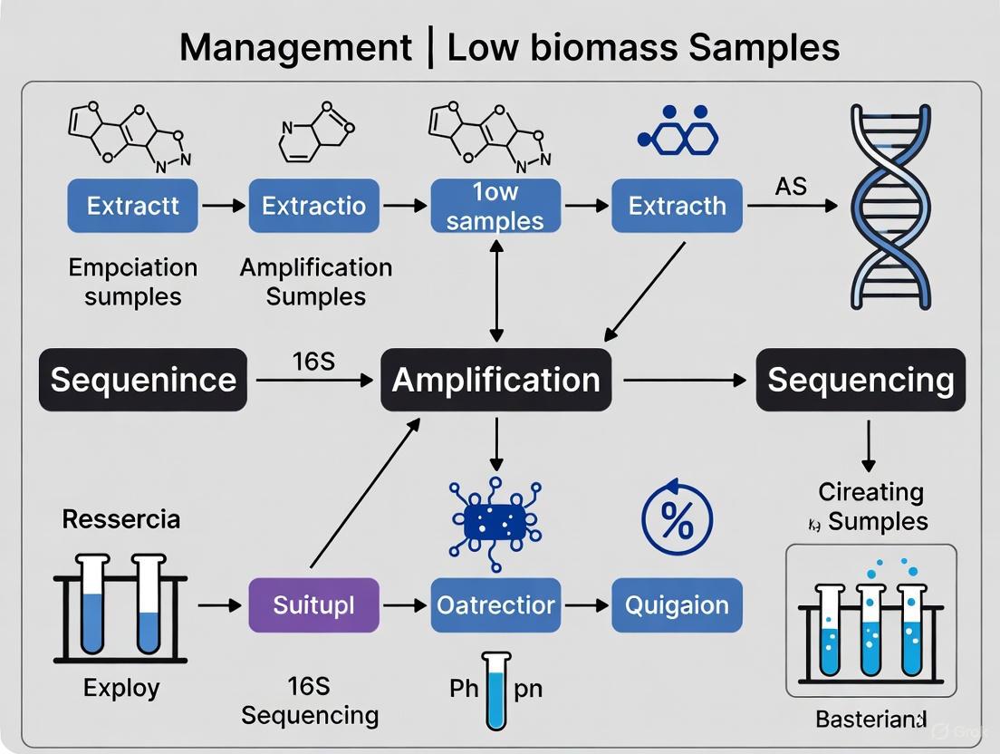
Experimental Protocol: A Rigorous Workflow for 16S rRNA Gene Sequencing of Low-Biomass Samples
The following protocol, synthesizing best practices from recent literature, is designed for processing respiratory (e.g., nasopharyngeal) or tissue biopsy samples [3] [8].
Step 1: Sample Collection & Nucleic Acid Extraction
Goal: Minimize contamination introduction during sample acquisition and DNA isolation.
- Collection: Use single-use, DNA-free collection vessels and swabs. Personnel should wear appropriate personal protective equipment (PPE) including gloves, masks, and clean lab coats to reduce contamination from skin and aerosols [1].
- Storage: Preserve samples in a suitable DNA-stabilizing buffer. PrimeStore Molecular Transport Medium has been shown to yield lower levels of background OTUs compared to other buffers like STGG [8].
- Extraction: Choose a kit validated for low-biomass samples. The NAxtra nucleic acid extraction protocol, which uses magnetic nanoparticles, has been piloted for respiratory samples and can be automated for high-throughput processing, completing extraction for 96 samples in approximately 14 minutes [3]. Alternatively, the DSP Virus/Pathogen Mini Kit (Kit-QS) has been shown to better represent hard-to-lyse bacteria compared to other kits like the ZymoBIOMICS DNA Miniprep Kit (Kit-ZB) [8].
- Elution: Elute DNA in a small volume (e.g., 50-80 µL) to increase DNA concentration for downstream steps [3].
Step 2: Library Preparation with Controls
Goal: Generate sequencing libraries while tracking and controlling for contaminants.
- PCR Amplification: Amplify the target 16S rRNA gene region (e.g., V1-V2 or V3-V4). For low-biomass samples, evidence suggests that conducting a single PCR reaction per sample (as opposed to pooling multiple PCR replicates) does not significantly impact outcomes like alpha and beta diversity, thereby saving time and resources [5].
- Mastermix: Using a premixed mastermix (vs. manually prepared) is acceptable and does not introduce significant bias, simplifying liquid handling [5].
- Inclusion of Controls: This is non-negotiable. Include the following in every run [1] [8] [2]:
- Negative Controls: No-template controls (NTCs, e.g., water), extraction blanks, and collection kit blanks.
- Positive Controls: A mock microbial community with a known composition (e.g., ZymoBIOMICS Microbial Community DNA Standard). This controls for amplification efficiency and bioinformatics accuracy.
- Technical Repeats: Process a subset of samples in duplicate or triplicate to assess reproducibility.
Step 3: Sequencing & Bioinformatics Analysis
Goal: Generate and analyze sequence data to distinguish biological signal from noise.
- Sequencing: Sequence on an Illumina MiSeq or similar platform. A sequencing depth of 50,000 reads per sample may be sufficient for low-biomass respiratory samples [3].
- Bioinformatics Processing: Use a standardized pipeline like QIIME 2. Key steps include:
- Denoising: Use DADA2 to infer amplicon sequence variants (ASVs) [3].
- Taxonomic Classification: Classify ASVs using a classifier (e.g.,
classify-sklearnin QIIME2) against a reference database (e.g., SILVA) [6]. Avoid open-reference clustering with low identity thresholds, as this reduces taxonomic resolution [6]. - Decontamination: Use statistical packages like
decontam(R) to identify and remove contaminants based on their prevalence in negative controls or their inverse correlation with DNA concentration [8]. Simply subtracting taxa found in NTCs is not recommended, as it can remove true biological sequences that have spilled over into controls via well-to-well contamination [8].
The following diagram visualizes the core workflow and the critical control points integrated at each stage.
The Scientist's Toolkit: Essential Reagents & Materials
Table 3: Key Research Reagent Solutions for Low-Biomass Studies
| Item | Function & Importance | Examples & Notes |
|---|---|---|
| DNA Decontamination Reagents | To remove contaminating DNA from surfaces and reusable equipment prior to sampling. Critical for reducing background noise [1]. | Sodium hypochlorite (bleach), UV-C light, hydrogen peroxide, DNA removal solutions. Note: Autoclaving and ethanol kill cells but may not remove persistent DNA [1]. |
| DNA-Free Collection Consumables | To collect samples without adding contaminating DNA. | Single-use, pre-sterilized swabs, collection tubes, and suction devices (e.g., SALSA sampler for surfaces) [1] [4]. |
| Nucleic Acid Extraction Kits | To isolate maximal microbial DNA from a minimal starting biomass. | Kits optimized for low biomass: NAxtra kit (magnetic nanoparticles), DSP Virus/Pathogen Mini Kit (Kit-QS) [3] [8]. |
| Mock Microbial Community | A positive control containing known microbes. Validates the entire workflow from extraction to sequencing [8] [5]. | ZymoBIOMICS Microbial Community DNA Standard; helps identify kit-specific contaminants ("kitome") and PCR biases [3] [5]. |
| Premixed PCR Mastermix | A consistent, ready-to-use reagent for amplification. Reduces liquid handling errors and contamination risk [5]. | Q5 Hot Start High-Fidelity 2× Mastermix; shown to perform equivalently to manually prepared mastermix for 16S rRNA gene sequencing [5]. |
FAQ: How Can I Visually Assess and Troubleshoot Contamination in My Data?
Effective troubleshooting involves both visual data exploration and statistical tests.
- Examine Control Samples in Ordination Plots: Plot your beta diversity (e.g., PCoA based on Bray-Curtis dissimilarity). If your negative controls (NTCs, blanks) cluster closely with or within your low-biomass experimental samples, it indicates that contamination is heavily influencing your experimental samples [8] [7].
- Check the Abundance of Known Contaminants: Review the taxonomic composition of your controls. Common reagent contaminants include Cutibacterium acnes, Pseudomonas, Acinetobacter, and Ralstonia [4] [5]. If these taxa are abundant in your controls and also appear in your experimental samples, they are likely contaminants.
- Use Prevalence-Based Decontamination: Employ the
decontampackage in R with the "prevalence" method. This method identifies taxa that are significantly more prevalent in negative controls than in true samples, providing a statistically robust way to flag contaminants for removal [8]. - Assess Biomass Correlation: For samples with quantified 16S copy numbers (e.g., via qPCR), the
decontam"frequency" method can identify contaminants based on their inverse correlation with total biomass [8].
This technical support center provides guidance for researchers working with low microbial biomass samples, where the total bacterial cell count is near or below the detection limits of standard protocols. A primary challenge in this field is establishing a critical biomass threshold—the minimum number of bacterial cells required to generate robust, reproducible, and accurate 16S rRNA gene sequencing data that reflects the true biological signal and is not overwhelmed by technical noise and contamination [9].
What is the Critical Biomass Threshold? Experimental evidence indicates that this threshold is approximately 10^6 bacterial cells [9]. Samples with biomass below this level consistently lose compositional accuracy and show significantly reduced reproducibility in duplicate or triplicate processing [10] [9].
Why is this Threshold Critical? In low biomass conditions, the absolute amount of target microbial DNA is vanishingly small. Consequently, even trace amounts of contaminating DNA from reagents, kits, or the laboratory environment can constitute a large proportion of the total sequenced DNA, leading to spurious results [1] [10]. Adhering to this validated threshold is therefore essential for producing credible data.
Frequently Asked Questions (FAQs)
FAQ 1: What is the definitive evidence for a 10^6 bacterial cell minimum? The most direct evidence comes from a systematic dilution study using stool samples from healthy donors and a mock microbial community [9]. Researchers created samples with precisely defined microbial loads, from 10^4 to 10^8 cells, and processed them using multiple DNA extraction and PCR protocols. The key finding was that samples containing 10^6 or fewer microbes lost their sample identity in cluster analysis, meaning their microbial composition profiles no longer reliably grouped with higher biomass replicates of the same origin. This effect was observed across different protocols, establishing 10^6 as a robust lower limit for reliable analysis [9].
FAQ 2: My samples are biopsies/swabs and likely have low biomass. What are my biggest risks? Working with low biomass specimens like biopsies and swabs introduces several critical risks that can compromise your data [1] [10]:
- Contaminant Dominance: Contaminating DNA from reagents, kits, and the lab environment will make up a larger proportion of your final sequencing library, potentially obscuring or mimicking a true biological signal [10].
- Cross-Contamination: DNA can "spill over" between samples during plate-based setup, especially from high-biomass samples to adjacent low-biomass wells. This is also known as well-to-well contamination [1] [10].
- Reduced Reproducibility: Technical replicates (sample processed in duplicate/triplicate) of low biomass specimens show much lower concordance than high biomass replicates, indicating results are not reliable [10].
- PCR Amplification Bias: At low template concentrations, stochastic effects and primer bias during PCR amplification are exaggerated, distorting the true relative abundances of taxa [9].
FAQ 3: How can I estimate the biomass in my sample before sequencing? While exact cell counts may require culture, you can use quantitative PCR (qPCR) to estimate the number of 16S rRNA gene copies in your extracted DNA, which serves as a proxy for bacterial load [11] [10]. One study defined low biomass technical repeats specifically as those represented by less than 500 16S rRNA gene copies per microlitre of sample [10]. Quantifying your DNA extract this way provides a crucial pre-sequencing check to gauge potential data quality issues.
FAQ 4: Are some DNA extraction kits better for low biomass work? Yes, the choice of DNA extraction method significantly impacts results. Studies comparing kits have found that protocols based on silica membrane columns (e.g., ZymoBIOMICS DNA Miniprep Kit) generally perform better for low biomass samples compared to bead absorption or chemical precipitation methods, both in terms of DNA yield and more accurate representation of the microbial composition [9]. Furthermore, increasing the mechanical lysing time during extraction can improve the lysis of hard-to-lyse bacteria (e.g., Gram-positives), leading to a more representative profile [9].
Troubleshooting Guides
Issue: High Background Noise in Sequencing Data
Problem: Sequencing data from low biomass samples shows a high abundance of taxa typically associated with contaminants (e.g., Pseudomonas, Acinetobacter, Ralstonia), and the profile looks similar to your negative controls.
Solutions:
- Intensify Pre-sequencing Decontamination: [1]
- Decontaminate all surfaces and equipment with 80% ethanol (to kill cells) followed by a nucleic acid degrading solution (e.g., dilute bleach or commercial DNA removal solutions) to destroy residual DNA.
- Use UV-irradiated, pre-cleaned plasticware and DNA-free reagents.
- Wear appropriate personal protective equipment (PPE) including gloves, mask, and clean suit to minimize human-derived contamination.
- Incorporate Comprehensive Controls: [1] [10]
- Negative Controls: Include multiple negative controls that mimic your entire experimental process. These should include "blank" extraction kits (adding only elution buffer) and "no-template" PCR controls.
- Positive Controls: Use a mock microbial community standard with a known composition and cell count at a level similar to your expected samples. This controls for both extraction efficiency and PCR bias.
- Apply In Silico Decontamination: Post-sequencing, use statistical tools like the
decontampackage in R to identify and remove sequences that are prevalent in your negative controls from your experimental samples [10]. This is more nuanced than simply subtracting a control profile.
Issue: Poor Reprobility Between Technical Replicates
Problem: When the same low biomass sample is processed in duplicate or triplicate, the resulting microbial community profiles are highly inconsistent.
Solutions:
- Verify Biomass Sufficiency: First, use qPCR to confirm your sample is at or above the 10^6 cell threshold. If it is consistently below this level, the fundamental issue may be insufficient starting material, and the experimental design may need revision [9].
- Optimize PCR Protocol: Switch from a standard PCR protocol to a semi-nested PCR approach. This has been shown to improve the sensitivity and reproducibility of 16S rRNA gene analysis for samples with low microbial biomass, allowing for more reliable profiling down to the 10^6 cell level [9].
- Minimize Cross-Contamination: Ensure physical separation during plate setup. Use sealed plates and be cautious of aerosol generation when handling samples post-amplification. Including a unique DNA spike-in control in each sample can also help monitor for well-to-well contamination [1] [11].
Experimental Protocols & Data
Validated Protocol for Low Biomass 16S rRNA Gene Analysis
The following workflow summarizes an optimized protocol, refined for low biomass samples, based on experimental evidence [9].
The table below consolidates key experimental findings that support the establishment of a 10^6 bacterial cell minimum.
Table 1: Experimental Evidence for the 10^6 Bacterial Cell Threshold
| Sample Type | Key Experimental Finding | Impact Below 10^6 Cells | Source |
|---|---|---|---|
| Healthy Donor Stool (Dilution Series) | Loss of sample identity in cluster analysis; profiles no longer group with higher biomass replicates. | Major: Inability to distinguish true biological differences from technical noise. | [9] |
| Bacterial Mock Community (Dilution Series) | Low biomass samples cluster midway between undiluted mock community and negative controls. | Major: True signal is lost and replaced by a hybrid of biology and contamination. | [10] |
| Nasopharyngeal & Induced Sputum | Technical replicates with low biomass (<500 16S copies/μL) showed higher alpha diversity and reduced reproducibility. | Major: Data becomes unreliable and non-reproducible. | [10] |
| Various (Theoretical Framework) | Maintenance metabolism converges on total metabolism for the smallest cells, highlighting extreme energy limitation. | Context: Explains the physiological challenge of being small and energy-limited. | [12] |
The Scientist's Toolkit: Essential Research Reagents & Materials
Table 2: Key Reagent Solutions for Low Biomass Research
| Item | Function & Importance | Specific Examples / Notes |
|---|---|---|
| Mock Microbial Community | A defined mix of bacterial cells or DNA used as a positive control to assess extraction efficiency, PCR bias, and sequencing accuracy. | ZymoBIOMICS Microbial Community Standard (D6300/D6305) [11] [13] [9]. |
| DNA Spike-in Control | A known quantity of foreign DNA (not found in your samples) added pre-extraction or pre-PCR to enable absolute quantification and monitor cross-contamination. | ZymoBIOMICS Spike-in Control I [11]. |
| Silica-Column DNA Extraction Kit | Provides high DNA yield and purity from low biomass samples; superior to bead absorption or chemical precipitation for this application. | ZymoBIOMICS DNA Miniprep Kit [9]; QIAamp PowerFecal Pro DNA Kit [11]. |
| DNA-Free Storage Buffer | Preserves sample integrity at collection while minimizing introduction of contaminating DNA. | PrimeStore Molecular Transport Medium [10]. |
| High-Fidelity Taq Polymerase | Reduces PCR amplification errors and bias, which is critical when amplifying tiny amounts of template DNA. | LongAmp Hot Start Taq DNA Polymerase [13]. |
| In Silico Decontamination Tool | A statistical software package to identify and remove contaminant sequences post-sequencing based on control samples. | Decontam (R package) [10]. |
FAQ: Where does contamination in 16S sequencing experiments primarily come from?
Contamination in 16S rRNA gene sequencing, especially for low-biomass samples, originates from several key sources. Reagents and laboratory environments introduce exogenous DNA that can be amplified and sequenced, obscuring the true biological signal.
- Reagents and Kits: DNA extraction kits, PCR master mixes, and molecular-grade water are well-documented sources of contaminating bacterial DNA. These often introduce a consistent set of bacterial taxa, sometimes called the "kitome" [14] [15].
- Laboratory Environment: Contaminants can be introduced from the air, lab surfaces, and equipment during sample processing [1] [14].
- Human Operators: Investigators can inadvertently introduce contamination from their skin, hair, or respiratory tract [1] [16].
- Cross-Contamination: This involves the transfer of DNA between samples during processing, a phenomenon known as well-to-well leakage [1] [17].
Table 1: Common Contaminant Genera and Their Sources
| Contaminant Genera | Typical Source |
|---|---|
| Pseudomonas, Ralstonia, Sphingomonas | Reagents (kits, water) [16] [15] |
| Acinetobacter, Herbaspirillum | Reagents (kits, water) [15] |
| Bacillus, Bradyrhizobium | Reagents (kits, water) [15] |
| Cutibacterium (formerly Propionibacterium) | Human skin, reagents [18] [16] |
| Stenotrophomonas | Reagents, and can also be a genuine pathogen [16] |
FAQ: How can I prevent contamination during sample collection and handling?
Preventing contamination begins at the sampling stage with strict sterile techniques and appropriate protective equipment.
- Use Single-Use, DNA-Free Consumables: Whenever possible, use pre-sterilized, disposable collection vessels and tools [1].
- Thorough Decontamination: Decontaminate reusable equipment and surfaces with 80% ethanol to kill microorganisms, followed by a DNA-degrading solution (e.g., sodium hypochlorite/bleach) to remove residual DNA [1].
- Wear Appropriate PPE: Wear gloves, lab coats, masks, and hair covers to minimize the introduction of human-associated contaminants. For extremely sensitive low-biomass work, more extensive cleanroom-style PPE may be necessary [1].
- Include Sampling Controls: Collect control swabs of the air in the sampling environment, PPE, or empty collection vessels. These controls help identify contaminants introduced during the collection process itself [1].
FAQ: What is the best experimental design to identify contamination in the lab?
A robust experimental design includes multiple types of controls processed alongside your biological samples through every step, from DNA extraction to sequencing.
- Negative Extraction Controls (NECs): These are "blank" samples where you substitute water or buffer for the biological sample during DNA extraction. They are essential for identifying contaminants from extraction kits and reagents [18] [16] [10].
- No-Template Controls (NTCs): Also known as library controls, these use water instead of DNA template during the PCR amplification step. They help identify contaminants present in PCR reagents, such as polymerases and buffers [19] [16].
- Mock Communities: These are commercially available or internally generated mixtures of known bacteria at defined ratios. They serve as positive controls to assess the accuracy and reproducibility of your entire workflow, from DNA extraction to sequencing [19] [10].
The following workflow outlines the key experimental and computational steps for managing contamination:
FAQ: How can I computationally remove contamination from my sequencing data?
After sequencing, bioinformatic tools can help identify and remove contaminant sequences. These methods typically use the control data you generated to distinguish contaminants from true biological signals.
- Frequency/Presence-Based Methods: Tools like the
decontampackage in R use the prevalence or relative abundance of Amplicon Sequence Variants (ASVs) in negative controls compared to true samples to classify contaminants [10] [17]. - Sample-Specific Thresholds: One approach suggests using the abundance of the most dominant contaminant species in your controls to set a sample-specific cutoff. Identifications below this threshold (e.g., 20% of the top contaminant's reads) are treated as potential contamination [18].
- Advanced Algorithms: Newer methods and packages are continuously being developed. For example,
micRocleanoffers pipelines for different research goals, andCleanSeqUis a recently developed algorithm that uses multiple rules, including Euclidean distance similarity and ecological plausibility, to decontaminate low-biomass urine data [17] [15]. - qPCR-Informed Decontamination: A powerful method combines sequencing data with quantitative PCR (qPCR) data measuring total bacterial load. It calculates the ratio of an OTU's "absolute" abundance (relative abundance × 16S gene copy number) in negative controls versus samples, effectively removing OTUs that are disproportionately abundant in controls [16].
Table 2: In Silico Decontamination Tools and Methods
| Tool / Method | Underlying Principle | Key Application / Note |
|---|---|---|
decontam (R package) |
Identifies contaminants based on higher prevalence or frequency in negative controls than in true samples [17]. | Widely used; combines control- and sample-based methods. |
| qPCR-Informed Pipeline | Uses bacterial load from qPCR to calculate "absolute" abundance ratio of OTUs in controls vs. samples [16]. | Removes OTUs disproportionately abundant in controls. |
micRoclean (R package) |
Houses two pipelines: "Original Composition" (estimates pre-contamination state) and "Biomarker" (strict removal) [17]. | Provides a filtering loss statistic to help avoid over-filtering. |
CleanSeqU Algorithm |
Classifies samples by contamination level and applies rules (Euclidean distance, Z-score, blacklist) [15]. | Specifically designed and validated for low-biomass urine samples. |
| Sample-Specific Cutoff | Uses the abundance of the top contaminant in a control to define a threshold for filtering in each clinical sample [18]. | A simple, transparent method not requiring specialized software. |
The Scientist's Toolkit: Key Reagent Solutions
Table 3: Essential Materials for Contamination-Aware 16S Sequencing
| Item | Function & Importance | Example / Note |
|---|---|---|
| DNA Extraction Kit | Extracts microbial DNA; a major source of the "kitome." Different kits have different contaminant profiles and lysis efficiencies [14] [10]. | DNeasy Kit (Qiagen), DSP Virus/Pathogen Mini Kit, ZymoBIOMICS DNA Miniprep Kit [14] [10]. |
| Sample Storage Buffer | Preserves sample integrity at the collection point. The choice of buffer can influence background contamination levels [10]. | PrimeStore Molecular Transport Medium, Skim-milk Tryptone Glucose Glycerol (STGG) [10]. |
| PCR Master Mix | Enzymes and buffers for amplification; a known source of contaminating DNA [14] [15]. | Use high-quality mixes and include NTCs. LongAmp Hot Start Taq Master Mix is used in the Nanopore 16S protocol [20]. |
| 16S Barcoding Primers | Allow multiplexing of samples; unique barcodes per sample are essential to track samples and identify cross-contamination [20] [19]. | e.g., the 24 unique barcodes in the Oxford Nanopore 16S Barcoding Kit [20]. |
| Nucleic Acid Cleanup Beads | Purify DNA and perform size selection to remove unwanted products like primer dimers. Incorrect ratios can cause sample loss or failure to remove small fragments [21] [20]. | AMPure XP Beads are commonly used [20]. |
| Mock Community | A defined mix of bacterial strains used as a positive control to validate the entire workflow's accuracy and reproducibility [19] [10]. | ZymoBIOMICS Microbial Community Standard, BEI Mock Bacterial Community [10]. |
How Low Biomass Amplifies Contaminant Signals and Skews Community Profiles
Troubleshooting Guides
Guide 1: Diagnosing and Correcting Contamination in Low-Biomass 16S rRNA Sequencing
Problem: Your 16S rRNA sequencing results from low-biomass samples (e.g., tissue, blood, urine) show unexpected microbial communities, high alpha diversity, or known common contaminants.
Explanation: In low-biomass environments, the small amount of target microbial DNA is easily overwhelmed by contaminant DNA from reagents, kits, and the laboratory environment [22] [23]. These contaminants constitute a larger proportion of the total DNA in your sample, distorting the true community profile and leading to inflated diversity metrics [22] [24]. Failure to account for this can lead to incorrect biological conclusions [1].
Solution: A multi-pronged approach combining rigorous lab practices and computational decontamination is required.
Step 1: Implement Robust Experimental Controls. Include the following controls in your sequencing run to identify contaminant signals [1] [2]:
- Negative Controls: DNA extraction blanks (e.g., an empty tube or tube with sterile water processed through extraction) and no-template PCR controls [22] [23].
- Positive Controls: A dilution series of a mock microbial community with a known composition [22] [5]. This helps evaluate the performance of your wet-lab and computational methods as microbial biomass decreases.
- Process-Specific Controls: Collect and sequence samples from potential contamination sources, such as swabs of sampling equipment, gloves, or aliquots of preservation solutions [1].
Step 2: Apply Computational Decontamination. Use your negative controls to filter out contaminants bioinformatically. The table below compares common methods:
| Method | Principle | Best Use Case | Key Limitation |
|---|---|---|---|
Decontam (Frequency) |
Identifies sequences with an inverse correlation to sample DNA concentration [22]. | General use; does not require prior knowledge of the environment [22]. | Requires DNA concentration data for all samples [22]. |
Decontam (Prevalence) |
Identifies sequences that are more prevalent in negative controls than in true samples [22]. | When you have multiple negative controls [22]. | May misclassify rare but true taxa if they appear in controls [22]. |
SourceTracker |
Uses a Bayesian approach to predict the proportion of a sample arising from defined contaminant sources [22]. | When the experimental environment is well-defined and source environments are known [22]. | Performs poorly when the experimental environment is unknown [22]. |
| Simple Subtraction | Removes all sequences found in negative controls from all samples [22]. | Quick, simple filtering. | Overly strict; can erroneously remove >20% of expected sequences present in controls due to index-hopping or other artifacts [22]. |
- Step 3: Set Sample-Specific Abundance Thresholds. For clinical diagnostics, one effective strategy is to use the most abundant contaminant species in your controls to set a filter. Reliable identifications in a sample should be above the read abundance of the most dominant contaminant found in that sample's associated controls [18].
Guide 2: Addressing Poor Library Yield and Quality from Low-Biomass Inputs
Problem: Your NGS library preparation from low-biomass samples results in low yield, high adapter-dimer formation, or poor library complexity.
Explanation: Low-input DNA increases the impact of common library prep issues. Suboptimal DNA quality, contaminants inhibiting enzymes, and over-amplification during PCR become major problems [21].
Solution: Systematically optimize each step of your library preparation protocol.
Step 1: Verify Input DNA Quality and Purity.
- Mechanism: Residual salts, phenol, or guanidine from extraction can inhibit enzymes used in fragmentation, ligation, and PCR [21].
- Action: Use fluorometric quantification (e.g., Qubit) instead of UV absorbance (NanoDrop) to accurately measure usable DNA. Check 260/230 and 260/280 ratios to ensure purity [21].
Step 2: Optimize Amplification to Reduce Bias.
- Mechanism: Too many PCR cycles can lead to over-amplification artifacts, chimeras, and a high duplicate rate, skewing representation [21] [5].
- Action: Use the minimum number of PCR cycles necessary. Evaluate whether pooling multiple PCR replicates per sample is necessary for your specific sample type, as it may not always be required and increases handling [5].
Step 3: Fine-Tune Purification and Size Selection.
- Mechanism: Aggressive clean-up can lead to loss of already scarce DNA fragments. An incorrect bead-to-sample ratio can fail to remove adapter dimers or exclude desired fragments [21].
- Action: Precisely follow bead-based clean-up protocols regarding ratios and incubation times. Avoid over-drying beads, which leads to inefficient resuspension and DNA loss [21].
Frequently Asked Questions (FAQs)
What defines a "low-biomass" sample, and why is it so problematic?
A low-biomass sample contains a very low concentration of microbial cells or DNA, placing it near the limits of detection for standard sequencing methods [1]. While sometimes defined quantitatively (e.g., <10,000 microbial cells/mL), it's best considered a continuum [2]. Examples include human tissues (blood, lung, placenta), certain environmental samples (drinking water, deep subsurface), and clinical specimens from normally sterile sites [24] [1]. The problem is proportional: the contaminant DNA "noise" can be as loud as, or louder than, the biological "signal," leading to distorted community profiles and inflated diversity estimates [22] [23].
Contamination can be introduced at virtually every stage of a study:
- Reagents and Kits: DNA extraction kits, PCR master mixes, and water are well-documented sources of bacterial DNA [5] [23].
- Laboratory Environment and Personnel: Human skin and hair, aerosols from talking, and laboratory surfaces are significant sources [1] [23].
- Sampling Equipment: Collection tubes, swabs, and solutions can introduce contaminants during sample acquisition [1].
- Cross-Contamination (Well-to-Well Leakage): DNA can transfer between samples on a 96-well plate during processing, a phenomenon known as the "splashome" [2].
How many negative controls should I include, and what kind?
There is no universal consensus on the number, but two controls are always better than one, and in some cases, more are helpful [2]. You should collect process controls that represent different contamination sources [2]. We recommend:
- Full-process controls that pass through the entire experiment (e.g., an extraction blank) to capture the aggregate contamination [2].
- Process-specific controls to identify specific sources (e.g., swab the collection kit, sample the preservation solution, swab the gloves of the operator) [1] [2]. This allows for more precise identification of contaminants.
Can't I just remove sequences that show up in my negative controls?
Simple subtraction is a common but flawed approach. While it seems straightforward, it can be too strict. It may erroneously remove over 20% of expected, true sequences that are also present in the negative control due to index-hopping or other low-level artifacts [22]. More sophisticated statistical methods like Decontam or SourceTracker are generally recommended as they can more accurately distinguish between contaminants and true signals [22].
Contamination has fueled several major controversies in microbiome research. For example, early claims of a distinct placental microbiome were later shown to likely be the result of contamination from reagents and laboratory processing, as the signal was indistinguishable from negative controls [1] [23]. Similarly, studies of blood and tumors have been debated due to the challenges of distinguishing ultra-low biomass signals from contamination [1] [2]. If contamination is confounded with a study group (e.g., all cases processed in one batch and all controls in another), it can create artifactual "associations" between contaminants and the disease state [2].
Experimental Protocols
Sample Collection & DNA Extraction for Low-Biomass Upper Respiratory Tract (URT) Samples
This protocol is adapted from best practices for microbial profiling of low-biomass upper respiratory tract samples [25].
Key Reagent Solutions:
- DNA-Free Swabs & Collection Tubes: Pre-sterilized, single-use to avoid introducing contaminants.
- Lysis Buffer (with mechanical lysis): A chemical lysis buffer, used in conjunction with a mechanical lysis step (e.g., bead beating with Lysing Matrix E) to ensure efficient cell wall disruption of hardy bacteria [5].
- DNA Extraction Kit: Use a kit designed for low-biomass samples. Include an extraction blank control (lysis buffer only) for every batch.
- Nuclease-Free Water: Certified DNA-free for all PCR and dilution steps.
- Mock Community DNA: A standardized community of known composition (e.g., ZymoBIOMICS Microbial Community Standard) to be used as a positive control [5].
Procedure:
- Sample Collection: Using sterile gloves and aseptic technique, collect the URT sample (e.g., nasal swab). Place the swab immediately into a DNA-free storage tube.
- Storage: Store samples at -70°C or in a preservation solution that stabilizes DNA until extraction.
- Nucleic Acid Extraction:
- Add samples to a tube containing a mechanical lysis matrix (e.g., Lysing Matrix E).
- Add lysis buffer and process on a homogenizer instrument (e.g., MPure-12 instrument) for mechanical disruption.
- Complete the DNA extraction following the manufacturer's protocol for the chosen kit.
- CRITICAL: Process your negative control (extraction blank) and positive control (mock community) alongside the experimental samples in the same batch.
- DNA Quantification: Quantify the extracted DNA using a fluorometric method (e.g., Qubit) for accuracy.
Evaluating Decontamination Methods Using a Mock Community Dilution Series
This methodology allows for the empirical testing of computational decontamination tools [22].
Key Reagent Solutions:
- Mock Microbial Community: A defined mix of known bacterial strains (e.g., from ZymoBIOMICS or ATCC).
- Nuclease-Free Water: For creating serial dilutions.
- Standard 16S rRNA Gene Primers & Master Mix: For library preparation.
Procedure:
- Create a Dilution Series: Perform a serial dilution (e.g., 3-fold or 10-fold dilutions) of the mock community DNA to simulate a range of high-to-low microbial biomass [22].
- Sequence the Series: Subject the entire dilution series, alongside your negative controls (water blanks), to standard 16S rRNA gene sequencing.
- Bioinformatic Analysis:
- Process the raw sequencing data to generate amplicon sequence variants (ASVs).
- Apply different computational decontamination methods (e.g.,
Decontamprevalence and frequency methods,SourceTracker, simple subtraction) to the dataset.
- Evaluation:
- Compare the output of each method against the known composition of the mock community.
- Calculate the percentage of contaminant sequences correctly removed and, crucially, the percentage of expected sequences erroneously removed by each method [22]. This will allow you to select the optimal method and parameters for your specific study.
Visualizations
Diagram 1: Impact of Decreasing Biomass on Contaminant Proportion
Frequently Asked Questions
1. What are the primary sources of false positives in 16S sequencing of low-biomass samples? False positives primarily arise from two key technical issues:
- Index Hopping (Sample Index Misassignment): This occurs during sequencing when DNA fragments from one sample are misassigned to another sample in the same sequencing run. It is a significant problem on certain platforms, with reported rates as high as 5.68% on the Illumina NovaSeq 6000 compared to 0.08% on the DNBSEQ-G400 platform [26]. These are high-quality biological reads, so they cannot be filtered out by standard quality control or denoising algorithms [26].
- Laboratory Contamination: Contaminating DNA can be introduced from reagents (the "kitome"), the laboratory environment, or sampling equipment. In low-biomass samples, this contaminant DNA can constitute a large proportion of the final sequencing library, leading to the detection of microbes that were never part of the original sample [14] [10] [1].
2. How does the loss of sample identity impact my research conclusions? Loss of sample identity, through sample mix-ups or cross-contamination, compromises the integrity of your entire dataset. This can lead to:
- Incorrect correlations between microbial profiles and sample metadata (e.g., linking contaminant microbes to a specific disease state) [26].
- Fake ecological patterns, such as inflated alpha diversity in simple communities or underestimated diversity in complex ones [26].
- Biased inference of community assembly mechanisms and the identification of fake keystone species in network analyses [26].
3. What is the best way to identify contaminating sequences in my data?
The most robust method involves the use of negative controls (e.g., blank extraction kits, sterile swabs, molecular grade water) processed alongside your biological samples. The sequences found in these controls represent the "contaminant profile" of your lab and reagents. These profiles can then be identified and removed from your biological samples using statistical tools like the decontam package in R, which compares the frequency or prevalence of sequences in samples versus controls [14] [10].
4. My samples are very precious and have low DNA yield. Is there a sequencing method better suited for this? Yes, for low-biomass, degraded, or host-DNA-dominated samples, alternative methods like 2bRAD-M sequencing are highly effective. This method uses type IIB restriction enzymes to produce small, uniform fragments, reducing amplification bias and allowing for species-level profiling from as little as 1 pg of total DNA or samples with 99% host DNA contamination [27].
Comparison of Sequencing Platforms and Bioinformatics Tools
Table 1: Quantitative Comparison of Sequencing Platform Index Misassignment Rates [26]
| Sequencing Platform | Technology | Reported Index Misassignment Rate | Impact on Rare Taxa Detection |
|---|---|---|---|
| Illumina NovaSeq 6000 | Sequencing-by-Synthesis | 5.68% | High level of false positive rare taxa |
| DNBSEQ-G400 | Combinatorial Probe-Anchor Synthesis & DNA Nanoballs | 0.08% | Rare taxa more likely to be biologically relevant |
Table 2: Characteristics of Common OTU and ASV Algorithms [28]
| Algorithm | Type | Key Strength | Key Weakness |
|---|---|---|---|
| DADA2 | Denoising (ASV) | Consistent output, high resemblance to expected community | Tends to over-split biological sequences |
| UPARSE | Clustering (OTU) | Low error rates, high resemblance to expected community | Tends to over-merge distinct sequences |
| Deblur | Denoising (ASV) | Consistent output | Tends to over-split biological sequences |
| Opticlust | Clustering (OTU) | Iterative cluster quality evaluation | Tends to over-merge distinct sequences |
Experimental Protocols
Protocol 1: Implementing Synthetic Spike-In Controls for Sample Tracking [29]
Purpose: To unambiguously track sample identity and detect cross-contamination throughout the 16S rRNA gene amplicon sequencing workflow.
Materials:
- Synthetic 16S rRNA gene spike-in controls (e.g., Sample Tracking Mixes - STMs)
- Environmental or host DNA samples
Methodology:
- Design: Create a unique combinatorial Sample Tracking Mix (STM) for each sample. Each STM is an equimolar mixture of 3 synthetic 16S rRNA gene sequences that are not found in nature.
- Spike-In: Add a low abundance of the unique STM (e.g., ~5,000 copies per nanogram of sample DNA) to each sample at the very beginning of DNA extraction.
- Processing: Carry the spiked-in samples through the entire workflow: DNA extraction, PCR amplification, library preparation, and sequencing.
- Bioinformatic Analysis: After sequencing, map all reads to a database containing the synthetic spike-in sequences.
- Verification: The STM detected in each sequenced library must match the one added to the original sample. A mismatch indicates a sample swap; the presence of multiple STMs indicates cross-contamination.
Protocol 2: Using Negative Controls and the Decontam Package [14] [10]
Purpose: To identify and remove contaminating sequences from 16S rRNA gene sequencing data.
Materials:
- DNA extraction kits
- Sterile water or buffer for negative controls
- R statistical software with the
decontampackage installed
Methodology:
- Experimental Setup: Include multiple negative controls (NTCs) in your sequencing batch. These should be tubes containing only the reagents used for DNA extraction and library preparation, with no sample added.
- DNA Extraction and Sequencing: Process the negative controls alongside your biological samples through every step, from DNA extraction to sequencing.
- Generate OTU/ASV Table: Process your raw sequencing data to generate a feature table (OTU or ASV counts per sample).
- Run Decontam: In R, use the
decontamfunction. You can use either the "prevalence" method (which identifies sequences significantly more common in samples than in controls) or the "frequency" method (which identifies sequences with higher relative abundance in controls than in samples). - Filter Table: Remove the sequences identified as contaminants from your feature table before proceeding with downstream ecological analysis.
Research Reagent Solutions
Table 3: Essential Materials for Managing Low-Biomass Sequencing Studies
| Item | Function | Example Use Case |
|---|---|---|
| Commercial Mock Communities | DNA from known mixtures of microbial strains; used as a positive control to assess accuracy, reproducibility, and bias in the entire workflow [26] [10]. | Verifying that your wet-lab and bioinformatic pipeline correctly identifies expected taxa without introducing false positives. |
| Synthetic Spike-In Controls | Artificially designed DNA sequences not found in nature; used to track sample identity and quantify cross-contamination [29]. | Adding a unique DNA barcode to each sample to detect tube mislabeling or well-to-well contamination during PCR. |
| DNA-Free Nucleic Acid Removal Solutions | Reagents (e.g., bleach, specialized commercial solutions) to decontaminate surfaces and equipment of trace DNA [1]. | Wiping down workbenches, centrifuges, and other equipment before working with low-biomass samples to reduce environmental contamination. |
| Specialized DNA Extraction Kits for Low Biomass | Kits optimized for efficient lysis of hard-to-break cells and maximal recovery of minimal DNA. | Extracting DNA from samples with very few cells, such as skin swabs, filtered air, or clinical tissue biopsies. |
Troubleshooting Workflow Diagram
The diagram below outlines a logical workflow for diagnosing and addressing false positives and sample identity issues.
Building a Robust Low Biomass Protocol from Sample to Sequence
Frequently Asked Questions (FAQs)
Q1: What are the most effective chemical agents for decontaminating work surfaces and equipment against DNA contamination?
The most effective decontamination strategies, as determined by controlled studies, are those that degrade DNA rather than just disinfect. For cell-free DNA, sodium hypochlorite (bleach) solutions and Trigene were highly effective, leaving a maximum of only 0.3% recoverable DNA on plastic, metal, and wood surfaces. For cell-contained DNA in substances like blood, 1% Virkon was most effective, with a maximum of 0.8% of DNA recovered post-decontamination [30]. It is critical to note that sterility is not the same as being DNA-free; ethanol and autoclaving kill viable cells but may leave cell-free DNA intact. For critical decontamination, a two-step process is recommended: 80% ethanol (to kill organisms) followed by a nucleic acid degrading solution like sodium hypochlorite to remove DNA traces [1].
Q2: How should we handle sampling equipment and consumables to minimize contamination?
A contamination-informed sampling design is essential. The following steps should be taken:
- Use DNA-Free Consumables: Ideally, use single-use, DNA-free collection vessels and tools [1].
- Decontaminate Reusable Equipment: If reusable equipment is necessary, decontaminate thoroughly with 80% ethanol followed by a DNA-degrading solution like sodium hypochlorite [1]. Commercial DNA removal solutions are also an option [30].
- Proper Handling of Plasticware: Plasticware or glassware for sample collection or storage should be pre-treated by autoclaving or UV-C light sterilization and remain sealed until the moment of use [1].
- Pre-Treat Gloves: Gloves should be similarly decontaminated and should not touch anything before sample collection [1].
Q3: What types of controls are non-negotiable in a low-biomass 16S rRNA sequencing study?
Including the correct controls is paramount for interpreting data from low-biomass studies and for using computational decontamination tools effectively. The necessary controls are [1] [22] [31]:
- Negative Extraction Controls (Blanks): These contain no sample and are processed alongside your experimental samples through DNA extraction and library preparation. They identify contaminating DNA from reagents and kits.
- Sampling Controls: These can include swabs of the air in the sampling environment, an empty collection vessel, or aliquots of the preservation solution. They help identify contaminants introduced during the collection process itself.
- Positive Controls (Mock Microbial Communities): These are mixtures of known bacteria. A dilution series of a mock community is particularly valuable as it helps evaluate the success of contaminant identification methods and shows how decreasing biomass increases the relative impact of contamination [22].
Q4: My negative controls show bacterial sequences. How do I determine if these are also present in my true samples?
This is a central challenge in low-biomass research. Simply removing all sequences found in negative controls from your dataset can be too harsh, as it may errone remove genuine, low-abundance taxa [22]. The recommended approach is to use bioinformatic tools that can distinguish contaminants based on their patterns of abundance. The R package Decontam, for instance, can identify contaminant sequences based on their inverse correlation with DNA concentration (the "frequency" method) or their prevalence in negative controls compared to true samples [22]. Other tools like SourceTracker and the recently developed CleanSeqU algorithm also use control data to statistically identify and remove contaminant sequences while preserving true biological signals [15] [22].
Q5: Beyond chemicals, what PPE and physical barriers are necessary during sampling?
Personal protective equipment (PPE) acts as a critical physical barrier to prevent contamination from the investigator. The appropriate level of PPE depends on the biomass of the sample, but core principles include [1] [32]:
- Full Body Coverage: Wear coveralls or cleansuits, gloves, goggles, shoe covers, and face masks.
- Protection from Aerosols: PPE protects samples from human aerosol droplets generated by breathing or talking, as well as cells shed from skin, hair, and clothing [1].
- Cleanroom Standards: For extremely sensitive work (e.g., ancient DNA or cleanroom sampling), extensive PPE including face masks, full-body suits, visors, and multiple glove layers is standard to eliminate skin exposure [1].
Troubleshooting Guides
Problem: Inconsistent Microbiome Profiles Across Replicates of Low-Biomass Samples
Potential Cause: Cross-contamination between samples during processing or variable contamination from reagents.
Solutions:
- Review Laboratory Workflow: Implement a unidirectional workflow, using separate rooms or dead-air cabinets for pre- and post-PCR work [30]. Use aerosol-resistant pipette tips.
- Include More Controls: Increase the number of negative extraction controls to better account for the "rule of small numbers," where a limited number of controls may not capture all contaminants [15].
- Apply Computational Decontamination: Use a bioinformatic pipeline like
DecontamorCleanSeqUwith your negative control data to identify and remove contaminant sequences from your dataset [15] [22]. - Quantify Bacterial Load: Use qPCR to determine the 16S rRNA gene copy number in each sample. This quantitative data can be integrated with sequencing data to better identify contaminants, as their relative abundance is often inversely correlated with total bacterial load [16].
Problem: Known Reagent Contaminants Appear as Abundant Taxa in Samples
Potential Cause: The high sensitivity of 16S rRNA PCR can amplify trace DNA from reagents, which becomes dominant when the true biological signal is very low.
Solutions:
- Procure DNA-Free Reagents: Source molecular biology grade water and extraction kits that are certified DNA-free.
- Treat Reagents: If possible, pre-treat reagents with methods to degrade DNA, such as UV irradiation or DNase, though effectiveness can vary [22].
- Leverage Positive Controls: Use a dilution series of a mock community. This allows you to observe how contaminants increase as biomass decreases and to fine-tune your decontamination algorithm's parameters [22].
- Use Advanced Bioinformatics: Apply algorithms capable of identifying abundant contaminants. For example,
CleanSeqUuses Euclidean distance similarity to compare the compositional pattern of dominant taxa in samples and blank controls, effectively removing taxa that show a similar proportional pattern to the blank [15].
Experimental Protocols & Data
Detailed Protocol: qPCR-Assisted Decontamination of 16S rRNA Gene Amplicon Datasets
This protocol outlines a method for in silico decontamination that combines sequencing data with quantitative PCR to better distinguish contaminants from true signals [16].
Methodology:
- Sample Processing and qPCR: Extract DNA from your samples and negative controls. Perform qPCR targeting a segment of the 16S rRNA gene (e.g., the V3 region) using universal bacterial primers. Use a standard curve (e.g., from E. coli or S. aureus DNA) to estimate the 16S rRNA gene copy number in each sample and negative control.
- 16S rRNA Gene Amplicon Sequencing: Generate V3–V4 16S rRNA gene amplicons from the same DNA extracts and sequence them on an Illumina platform. Process the sequences through a standard pipeline (e.g., QIIME2 with DADA2) to generate an Amplicon Sequence Variant (ASV) table.
- In Silico Decontamination Calculation:
- For each ASV in each sample, calculate its "absolute" abundance in arbitrary units by multiplying its relative abundance (from the ASV table) by the 16S rRNA gene copy number for that sample (from qPCR).
- Calculate the ratio (R-OTU) for each ASV: (mean "absolute" abundance in negative controls) / (mean "absolute" abundance in true samples).
- Set a cutoff value for R-OTU (e.g., 0.01). Remove any ASV from the dataset where its R-OTU ratio exceeds this cutoff, as it is more abundant in controls than samples and is likely a contaminant.
Workflow Visualization:
Quantitative Data on Decontamination Efficiency
The table below summarizes the efficiency of various cleaning strategies for removing DNA from different surfaces, as recovered from contaminated surfaces post-cleaning [30].
Table 1: Efficiency of Cleaning Strategies for DNA Removal from Different Surfaces
| Cleaning Agent | Surface | Mean mtDNA Copies Recovered (Cell-Free DNA) | Percent Yield vs. Control (Cell-Free DNA) |
|---|---|---|---|
| No-treatment control | Plastic | 9,396,667 | 100.0% |
| Metal | 5,701,333 | 100.0% | |
| Wood | 4,792,667 | 100.0% | |
| 70% Ethanol | Plastic | 1,066,667 | 11.4% |
| Metal | 1,680,000 | 29.5% | |
| Wood | 1,436,000 | 30.0% | |
| UV Radiation | Plastic | 1,733,333 | 18.4% |
| Metal | 1,205,333 | 21.1% | |
| Wood | 1,140,000 | 23.8% | |
| 0.5% Sodium Hypochlorite (Fresh) | Plastic | 11,467 | 0.1% |
| Metal | 17,200 | 0.3% | |
| Wood | 3,333 | 0.1% | |
| 1% Virkon | Plastic | 29,867 | 0.3% |
| Metal | 13,067 | 0.2% | |
| Wood | 10,800 | 0.2% | |
| 10% Trigene | Plastic | 12,533 | 0.1% |
| Metal | 17,467 | 0.3% | |
| Wood | 5,467 | 0.1% |
The Scientist's Toolkit: Essential Research Reagent Solutions
Table 2: Key Reagents and Materials for Low-Biomass Sampling and Decontamination
| Item | Function / Explanation | Key Considerations |
|---|---|---|
| Sodium Hypochlorite (Bleach) | A highly effective DNA-degrading agent for surface decontamination [30]. | Prepare fresh dilutions for maximum efficacy; concentration of available chlorine decreases over time [30]. |
| DNA-Free Water | Used as a solvent for molecular biology reactions and for moistening swabs. | A common source of contaminating DNA; ensure it is certified DNA-free [15]. |
| Forensic-Grade Swabs | For sample collection from surfaces. | Use single-use, DNA-free swabs to avoid introducing contaminants [32]. |
| Personal Protective Equipment (PPE) | A physical barrier to prevent contamination from the investigator [1] [32]. | Should include gloves, mask, cleansuit, and hair cover. Change gloves frequently. |
| Negative Extraction Control | Contains no sample and is processed identically to true samples to identify reagent-derived contaminants [22] [16]. | Essential for all computational decontamination methods. |
| Mock Microbial Community | A defined mixture of known microorganisms used as a positive control [22] [31]. | A dilution series can be used to validate decontamination protocols and benchmark bioinformatic tools [22]. |
| qPCR Reagents | For quantifying total bacterial load via 16S rRNA gene copy number [16]. | This quantitative data can be combined with sequencing data to improve contaminant identification [16]. |
In 16S rRNA gene sequencing, particularly for low biomass samples, the DNA extraction method is not merely a preliminary step but a major determinant of experimental success. Low biomass samples—such as tissue swabs, biopsies, and human milk—contain few microbial cells, making the complete and unbiased lysis of those cells paramount. The method you choose directly impacts DNA yield, purity, and, most critically, the faithful representation of the microbial community. Inaccurate lysis can skew results, leading to the under-representation of tough-to-lyse Gram-positive bacteria and fundamentally altering the perceived microbial diversity [33] [9] [34]. This guide provides a technical deep dive into the performance of three core DNA extraction technologies—silica columns, bead-based, and chemical precipitation—to help you select and troubleshoot the optimal protocol for your low biomass research.
Methodology: How We Compare the DNA Extraction Methods
To ensure a fair and quantitative comparison, the performance of DNA extraction methods is typically evaluated using a combination of standardized samples and a set of wet- and dry-lab criteria.
Standardized Samples for Evaluation:
- Mock Communities: Defined mixtures of bacterial species with known abundances, including both Gram-positive and Gram-negative bacteria. These are the gold standard for assessing extraction accuracy and bias, as they allow for a direct comparison between observed sequencing results and the theoretical composition [33] [35] [34].
- Low Biomass Clinical Samples: Real-world samples like human milk, gill swabs, or stool dilutions are used to test protocol performance under realistic conditions where inhibitor content and host DNA contamination are challenges [9] [34] [36].
Performance Evaluation Criteria:
- Wet-Lab Metrics: DNA yield (concentration), DNA purity (A260/280 ratio), and DNA fragment size.
- Dry-Lab (Sequencing) Metrics: Alpha-diversity (a measure of within-sample diversity, correlated with effective lysis of Gram-positives), and accuracy in recovering the expected composition of mock communities [33] [9].
Table: Key Performance Metrics for DNA Extraction Method Evaluation
| Metric | Description | Why It Matters for Low Biomass |
|---|---|---|
| DNA Yield | Total quantity of DNA recovered | Critical for downstream library prep; low yield may fail to sequence. |
| DNA Purity (A260/280) | Ratio indicating protein or RNA contamination | Contaminants can inhibit enzymatic reactions in PCR and sequencing. |
| Fragment Size | Average length of extracted DNA fragments | Shorter fragments may indicate excessive shearing, affecting library quality. |
| Alpha-Diversity | Richness and evenness of species in a sample (e.g., Chao1, Shannon) | Under-lysed samples show artificially low diversity. |
| Taxonomic Accuracy | Fidelity in recovering expected mock community composition | Reveals bias against hard-to-lyse (e.g., Gram-positive) bacteria. |
Performance Showdown: A Quantitative Comparison
Independent studies have systematically compared these methods to uncover their strengths and weaknesses. The following table summarizes the typical performance characteristics of each method in the context of low biomass and complex samples.
Table: Direct Comparison of DNA Extraction Methods for 16S Sequencing
| Method | Mechanism | Best For | Pros | Cons |
|---|---|---|---|---|
| Silica Columns (e.g., QIAamp Stool Mini, DNeasy PowerSoil Pro) | DNA binds to silica membrane under high-salt conditions; washed and eluted. | Standardized processing; high purity needs [34]. | High purity; easy to automate; cost-effective for high-throughput [37]. | Can be biased if lysis is incomplete; may not recover all Gram-positives without bead-beating [33]. |
| Bead-Based / Bead-Beating (e.g., DNeasy PowerLyzer PowerSoil, ZymoBIOMICS) | Mechanical disruption via vigorous shaking with small beads. | Low biomass samples; tough-to-lyse Gram-positive bacteria [33] [9]. | Excellent for robust lysis of diverse cells; high yield and diversity [33]. | Can shear DNA if overdone; potential for inter-protocol variability [35]. |
| Chemical Precipitation (e.g., Phenol-Chloroform, Alkaline Lysis) | Organic extraction or alkaline denaturation to separate DNA. | Budget-conscious labs; specific Gram-positive targets (alkaline method) [35]. | No specialized equipment needed; effective on some tough cells [35]. | Toxic reagents (phenol); complex, manual steps; lower purity [37]. |
Key Research Findings:
- Bead-Beating Enhances Diversity: A 2023 study comparing four DNA extraction methods for gut microbiome analysis found that protocols incorporating bead-beating (e.g., DNeasy PowerLyzer PowerSoil) consistently yielded higher observed microbial alpha-diversity, which is strongly correlated with the effective lysis of Gram-positive bacteria [33].
- The Low Biomass Limit: Research from 2021 demonstrated that sample biomass itself is a primary limiting factor. For 16S rRNA gene analysis to be robust and reproducible, a minimum of 10^6 bacterial cells per sample is required. Below this threshold, sample identity is lost, regardless of the extraction method used [9].
- The "Rapid" Alkaline Method: A novel, non-bead-beating method using potassium hydroxide (KOH), heat, and detergent showed promise in 2024. This "Rapid" protocol provided consistent representation of both easily lysed and difficult-to-lyse bacteria, recovering higher levels of Firmicutes (Gram-positives) in mock communities and human fecal samples compared to some standard protocols [35].
- Kit Performance in Human Milk: A 2023 study on human milk microbiome identified the DNeasy PowerSoil Pro (bead-based) and MagMAX Total Nucleic Acid Isolation (magnetic bead-based) kits as providing the most consistent 16S rRNA gene sequencing results with the lowest levels of contamination, a critical factor for low biomass samples [34].
Troubleshooting Guide & FAQs
Frequently Asked Questions
Q1: My DNA yield from a low biomass swab sample is too low for library prep. What can I do?
- A: First, confirm the problem. Use a fluorescence-based assay for quantification, as it is more accurate for low-concentration samples. Consider switching to a bead-beating protocol, as it generally provides higher yields and better lysis efficiency. For very precious samples, you can use a whole genome amplification kit, but be aware this may introduce bias [9]. Optimizing sample collection to maximize bacterial recovery and minimize host DNA—for example, using surfactant-based washes instead of whole tissue—can dramatically improve 16S rRNA gene recovery [36].
Q2: My DNA purity (A260/A280) is low. What does this indicate and how can I fix it?
- A: A low A260/A280 ratio (<1.8) typically indicates protein contamination. Ensure you are using the correct lysis conditions and that all washing steps are thoroughly performed. A high ratio (>2.0) may suggest RNA contamination, which can be mitigated by adding an RNase A digestion step during extraction [33] [38].
Q3: Why is my microbial diversity lower than expected, and how is it related to DNA extraction?
- A: Low diversity often stems from incomplete cell lysis. Gram-positive bacteria with thick peptidoglycan layers are frequently under-represented in gentle lysis protocols. The solution is to incorporate a mechanical lysis step, such as bead-beating. Studies show that increasing mechanical lysing time and repetition ameliorates the representation of bacterial composition [33] [9].
Q4: I'm seeing a lot of contamination in my negative controls. What is the source?
- A: Contamination in low biomass studies is a major challenge. Sources can include reagents, kits, and the laboratory environment. Always include negative control samples (e.g., blank extractions with water) to identify contaminating sequences. Using UV-irradiated benches, dedicated equipment, and commercially verified low-biomass kits can help mitigate this issue [34] [39].
Essential Protocols for Your Research
Detailed Protocol: Bead-Beating Extraction for Low Biomass Samples (based on DNeasy PowerLyzer PowerSoil Kit)
This protocol is recommended for its robust lysis and reproducibility with low biomass samples [33] [34].
- Sample Preparation: Centrifuge your sample (e.g., 3.5 mL of human milk) at 13,000-20,000 × g for 15 minutes at 4°C. Carefully remove the fat layer and supernatant.
- Initial Lysis: Resuspend the pellet in the provided Solution CD1 and transfer it to a PowerBead Pro tube.
- Bead-Beating: Lyse cells using a homogenizer (e.g., Precellys Evolution) at 5000 rpm for 45-60 seconds. Keep samples cool at 4°C during beating to prevent DNA degradation.
- Centrifugation: Centrifuge the tubes at 15,000 × g for 1 minute to pellet debris.
- DNA Binding and Washing: Transfer the supernatant to a new tube and complete the DNA purification according to the manufacturer's instructions, using a silica-based membrane column. This includes binding, washing with ethanol-based buffers, and a final dry spin.
- Elution: Elute the pure genomic DNA in a low-EDTA TE buffer or nuclease-free water. Store at -20°C or -80°C.
Detailed Protocol: Rapid Alkaline Lysis for Milligram Quantities
This is a simplified, non-mechanical protocol suitable for milligram-scale samples when bead-beaters are unavailable [35].
- Sample Input: Transfer ≤10 mg of sample (e.g., fecal material) to a 1.5 mL tube.
- Chemical Lysis: Add a pre-prepared lysis buffer containing potassium hydroxide (KOH), a detergent, and heat to 95°C. Vortex thoroughly to homogenize.
- Incubation: Incubate the sample at 95°C for 10 minutes to facilitate complete cell wall disruption and DNA release.
- Neutralization and Dilution: Dilute the lysate with a neutralization buffer to reduce the pH and ionic strength, making it compatible with downstream PCR.
- Direct Use: The diluted lysate can be used directly as a template in 16S rRNA gene PCR amplification without further DNA purification.
The Scientist's Toolkit: Key Reagents & Solutions
Table: Essential Research Reagents for DNA Extraction from Low Biomass Samples
| Reagent / Kit | Function | Application Note |
|---|---|---|
| DNeasy PowerSoil Pro Kit (QIAGEN) | Bead-beating and silica column purification. | Recommended for low biomass human milk and environmental samples; effective inhibitor removal [34]. |
| ZymoBIOMICS DNA Miniprep Kit (Zymo Research) | Bead-beating and silica column purification. | Effective for a wide range of biomasses down to 10^4 microbes; includes DNA cleanup [9]. |
| Mock Microbial Community (ZymoBIOMICS) | Defined standard for validating extraction bias and sequencing accuracy. | Contains both Gram-positive and Gram-negative bacteria to test lysis efficiency [35] [34]. |
| Proteinase K | Enzyme that digests proteins and degrades nucleases. | Critical for lysis of animal tissues and inactivation of DNases; add before lysis buffer [38] [37]. |
| Lysis Buffer (with KOH) | Alkaline solution that denatures membranes and proteins. | Core of the "Rapid" protocol; effective on tough Gram-positive cell walls [35]. |
| Silica Magnetic Beads | Solid-phase for DNA binding and purification in solution. | Enables automation on liquid handling robots; no centrifugation required [37] [40]. |
Workflow Visualization: Choosing Your Extraction Method
The following diagram illustrates the decision-making process for selecting the most appropriate DNA extraction method based on your sample type and research goals.
Frequently Asked Questions (FAQs)
FAQ 1: Why is mechanical lysis, specifically bead beating, considered critical for 16S rRNA gene sequencing from low-biomass samples?
Mechanical lysis is considered the gold standard for microbiome DNA extraction because it provides a stochastic and unbiased method for breaking open a wide range of bacterial cell types. Complex microbial communities inevitably contain tough-to-lyse species, such as Gram-positive bacteria with thick peptidoglycan cell walls, spores, and yeast [41]. If not lysed efficiently, these organisms will be underrepresented in the final sequencing data, leading to a skewed community profile. Methods that rely solely on chemical or thermal lysis often cause overrepresentation of easy-to-lyse organisms (e.g., Gram-negative bacteria) and poor liberation of DNA from tough-to-lyse organisms [41]. Bead beating's physical disruption helps ensure that DNA is released from both easy-to-lyse and recalcitrant microbes, which is paramount for an accurate representation of the true microbial community, especially in low-biomass samples where every cell counts [42] [33] [41].
FAQ 2: How do the duration and repetition of bead beating impact DNA yield, quality, and community representation?
The intensity and duration of mechanical lysis create a trade-off between DNA yield and DNA fragment length. Higher intensity (speed and time) generally increases DNA yield by lysing more cells but also shears DNA into shorter fragments, which can be detrimental for long-read sequencing technologies [43]. Conversely, lower energy input preserves longer DNA fragments but may reduce total yield [43].
Critically, the community representation can be significantly affected. One study on rumen samples found that including a bead-beating step increased total DNA yield but decreased the observed richness of protozoal amplicons [42]. However, another study on vaginal microbiota found that while different lysis methods (including bead beating) resulted in statistically significant differences in beta diversity, these differences were small compared to the biological variation between samples [44]. The optimal setting must therefore balance these factors for your specific sample type and downstream application.
Table 1: Impact of Bead Beating Intensity on DNA Yield and Fragment Length in Soil Samples [43]
| Homogenisation Parameters | Distance Travelled (m) | DNA Yield (Total µg) | Mean DNA Fragment Length (bp) |
|---|---|---|---|
| 4 m s⁻¹ for 5 s | 20 | ~2.5 | 9,324 |
| 4 m s⁻¹ for 10 s | 40 | Sufficient for sequencing | 7,487 |
| 6 m s⁻¹ for 30 s | 180 | ~4.0 | 4,406 |
| Higher Intensity Settings | 360 - 960 | Plateaued | 3,418 - 4,156 |
FAQ 3: Are there any validated protocols for bead beating that I can follow?
Yes, several studies and manufacturers have provided validated bead-beating protocols. Zymo Research, using their ZymoBIOMICS Microbial Community Standard, has extensively tested and published parameters for various homogenizers to ensure unbiased nucleic acid extraction with their ZymoBIOMICS DNA Miniprep Kit [41]. Furthermore, a 2023 study optimizing DNA extraction for the human gut microbiome found that a protocol combining a stool preprocessing device with the DNeasy PowerLyzer PowerSoil kit (which includes a bead-beating step) showed the best overall performance [33].
Table 2: Examples of Validated Bead Beating Protocols [41]
| Homogenizer | Recommended Protocol |
|---|---|
| MP Fastprep-24 | 1 minute at max speed, 5 minutes rest. Repeat cycle 5 times (total of 5 minutes bead beating). |
| Biospec Mini-BeadBeater-96 (with 2 ml tubes) | 5 minutes at Max RPM, 5 minutes rest. Repeat cycle 4 times (total of 20 minutes bead beating). |
| Bertin Precelys Evolution | 1 minute at 9,000 RPM, 2 minutes rest. Repeat cycle 4 times (total of 4 minutes bead beating). |
| Vortex Genie (with adapter) | 40 minutes of continuous bead beating (max 18 tubes). |
FAQ 4: What common issues should I troubleshoot if my 16S sequencing results show low diversity or underrepresentation of Gram-positive bacteria?
If your sequencing data shows low diversity or an unexpected lack of Gram-positive bacteria, the issue most likely lies with inefficient mechanical lysis.
- Problem: Underrepresentation of Gram-positive taxa.
- Potential Cause: The bead-beating step was not intense or long enough to break open the tough peptidoglycan layers of Gram-positive bacterial cell walls.
- Solution: Increase the intensity of mechanical lysis. This can be done by:
- Increasing the duration of the bead-beating cycles.
- Incorporating repeated cycles of beating with rest periods in between to prevent excessive heat buildup, as seen in the validated protocols above [41].
- Ensuring you are using the appropriate size and material of beads (e.g., a mix of zirconia/silica beads) to enhance lysis efficiency [33].
- Verification: Always include a mock community of known composition (e.g., ZymoBIOMICS Microbial Community Standard) in your extraction batches. If your results from the mock community do not match the expected composition, particularly for the tough-to-lyse species, it confirms a bias in your DNA extraction protocol that needs to be addressed [41] [10].
Experimental Protocols for Key Studies
This protocol uses a statistical design of experiments (DoE) approach to optimize mechanical lysis for maximum DNA fragment length from soil, which is directly applicable to other complex, low-biomass samples.
- Sample Preparation: Begin with 250 mg of soil sample.
- Homogenization: Use a benchtop homogenizer (e.g., FastPrep-24). The study found that the number of repeated cycles did not significantly impact results, so a single cycle is sufficient.
- Parameter Optimization: Systematically test different combinations of homogenization speed (e.g., 4 m s⁻¹ to 6 m s⁻¹) and total homogenization time (e.g., 5 s to 30 s).
- Key Finding: The optimized setting was 4 m s⁻¹ for 10 s, which increased the mean purified DNA fragment length by 70% compared to the manufacturer's standard recommendation (6 m s⁻¹ for 30 s), while still providing sufficient DNA yield for sequencing library preparation.
- DNA Purification: Proceed with the remainder of your chosen commercial soil DNA extraction kit protocol.
This protocol directly compares enzymatic and mechanical lysis pretreatments.
- Sample Aliquoting: Thoroughly mix the sample and divide it into multiple 100 µl aliquots.
- Lysis Pretreatments:
- Chemical/Enzymatic Lysis: Incubate aliquots with lysozyme (20 mg/ml) at 37°C for 30 minutes. Variations can include extended incubation (16 hours) or the addition of an enzyme cocktail (mutanolysin and lysostaphin).
- Mechanical Lysis: For the bead-beating condition, first subject an aliquot to 30 minutes of enzymatic lysis with lysozyme as above. Then, add ~200 mg of 0.1-mm-diameter zirconia/silica beads and process in a homogenizer (e.g., Tissue Lyser II) for 30 seconds at 25 Hz.
- DNA Extraction: After the pretreatment, add proteinase K and buffer AL from a commercial kit (e.g., Qiagen DNeasy Blood and Tissue kit) and continue with the standard extraction protocol.
- Key Finding: While the bead-beating method produced lower DNA yields, it did not significantly alter the observed alpha diversity compared to other methods. Beta diversity was significantly different but minor compared to sample-to-sample variation.
Workflow Diagram
The following diagram illustrates the decision-making process and trade-offs involved in optimizing a mechanical lysis protocol.
Research Reagent Solutions
Table 3: Essential Materials for Optimized Mechanical Lysis
| Item | Function/Description | Example Products/Brands |
|---|---|---|
| Bead Beating Homogenizer | Instrument for consistent and efficient mechanical cell disruption. | FastPrep-24 (MP Biomedicals), Mini-BeadBeater-96 (Biospec), Precelys Evolution (Bertin) |
| Lysis Tubes with Beads | Tubes containing beads of specific size and material to physically grind cells. | Zirconia/Silica beads (0.1 mm - 0.5 mm), BashingBead Tubes (Zymo Research) |
| DNA Extraction Kit (with beads) | Provides optimized buffers and columns for DNA purification post-lysis. | DNeasy PowerLyzer PowerSoil Kit (QIAGEN), ZymoBIOMICS DNA Miniprep Kit (Zymo Research) |
| Mock Microbial Community | Defined mixture of bacteria (Gram-positive and Gram-negative) to validate lysis efficiency and avoid bias. | ZymoBIOMICS Microbial Community Standard (Zymo Research), BEI Mock Community (BEI Resources) |
FAQ: Primer Selection and Performance
What is the core challenge with "universal" 16S rRNA primers?
The primary challenge is that widely used "universal" primers often fail to capture the full spectrum of microbial diversity due to unexpected variability in the conserved regions of the 16S rRNA gene where these primers are designed to bind [45]. This amplification bias arises because primers were historically designed based on limited datasets of culturable bacteria, which do not fully represent the diversity found in complex modern microbiome samples [45]. Consequently, specific but important taxa can be underrepresented or completely missed with unsuitable primer combinations [46].
How does target region selection (e.g., V1-V9 vs. V3-V4) impact my results?
The choice of variable region significantly influences the taxonomic composition you observe [46]. Different variable regions have varying sensitivities for discriminating closely related taxa, and the taxonomic resolution differs across bacterial phyla [46]. For instance:
- Full-length vs. Short-Amplicon: Sequencing the full-length 16S rRNA gene (V1-V9) with long-read technologies provides higher taxonomic resolution, potentially down to the species level. In contrast, short-read sequencing of regions like V3-V4 typically limits resolution to the genus level [47].
- Primer-Specific Biases: Microbial profiles cluster primarily by primer pair rather than by sample donor, and certain taxa may be uniquely detected or missed by specific primers. For example, the Bacteroidetes phylum can be missed when using primers 515F-944R (targeting V4-V5) [46].
What is primer degeneracy and why is it important?
Primer degeneracy involves incorporating multiple nucleotides at specific positions within the primer sequence to account for natural variations in the target gene across different bacteria. The degree of degeneracy is critical for coverage [47].
Comparative studies on full-length 16S rRNA sequencing have shown striking differences in results based on degeneracy. A conventional primer (27F-I) revealed a significantly lower biodiversity and an skewed community structure (e.g., dominance of Firmicutes and Proteobacteria, high Firmicutes/Bacteroidetes ratio) compared to a more degenerate primer set (27F-II). The more degenerate primer produced a microbial profile that better reflected the expected composition of a human gut microbiome [47].
How do I know if my primer choice is biasing my low-biomass results?
In low-biomass research, primer bias is compounded by contamination risks. Key indicators of potential bias include:
- Profiles Resembling Controls: Your sample profiles appear similar to your negative (no-template) controls [8].
- Inconsistent Replicates: Low reproducibility between technical replicates of the same sample [8].
- Unexpected Diversity: An unusually high alpha diversity in low-biomass samples, which can signal significant contaminant DNA amplification [8].
- Mismatch with Expected Biology: Results that contradict established biological knowledge for the sample type, which can be checked against large-scale projects like the American Gut Project [47].
What strategies can I use to validate and improve primer coverage?
- In-silico Validation: Before wet-lab work, use tools like TestPrime to evaluate primer performance against reference databases (e.g., SILVA) to predict coverage for your phyla of interest [45].
- Use Mock Communities: Always include mock communities of known composition and adequate complexity. They are essential for identifying biases in amplification, sequencing, and bioinformatic analysis [46] [8].
- Multi-Primer Approach: For critical findings, consider using a multi-primer strategy to amplify different variable regions, which can help mitigate the biases inherent in any single primer set [45].
- Database Consistency: Be aware that different reference databases (GreenGenes, SILVA, RDP) use different nomenclatures and curation. Use the same database consistently, especially when comparing datasets [46].
Technical Reference Tables
| Target Region | Example Primers | Typical Read Length | Key Advantages | Key Limitations & Biases |
|---|---|---|---|---|
| V1-V2 | 27F-338R | Short-amplicon | Commonly used for human gut samples [46]. | Differences in composition outcome; less pronounced at higher taxonomic levels [46]. |
| V3-V4 | 341F-785R | Short-amplicon | Most commonly used for Illumina MiSeq; well-established protocols [46]. | Limits taxonomic resolution to genus level at best; primer bias affects detected diversity [47]. |
| V4 | 515F-806R | Short-amplicon | Common, well-studied region [46] [25]. | Can miss specific taxa; overall diversity and abundance profiles can be skewed [46]. |
| V4-V5 | 515F-944R | Short-amplicon | Covers two variable regions. | Can miss entire phyla (e.g., Bacteroidetes) [46]. |
| V6-V8 | 939F-1378R | Short-amplicon | Covers multiple variable regions. | Can produce primer-specific profiles that are not comparable to other regions [46]. |
| Full-Length (V1-V9) | 27F-1492R | Long-amplicon (~1500 bp) | Highest taxonomic resolution (to species level); improves identification of novel taxa [47] [48]. | Requires third-gen sequencing (e.g., Nanopore); historically higher error rates (now <2%) [47]. |
Table 2: In-silico Coverage of Selected Primer Sets Across Dominant Gut Phyla
This table summarizes data from a systematic in-silico analysis of 57 primer sets, showing how even primers for the same region can have varying performance [45]. Coverage is defined as the percentage of eligible sequences in the SILVA database that are successfully amplified.
| Primer Set ID | Target Region | Approx. Coverage in Actinobacteriota | Approx. Coverage in Bacteroidota | Approx. Coverage in Firmicutes | Approx. Coverage in Proteobacteria |
|---|---|---|---|---|---|
| V3_P3 | V3 | ≥70% | ≥70% | ≥70% | ≥70% |
| V3_P7 | V3 | ≥70% | ≥70% | ≥70% | ≥70% |
| V4_P10 | V4 | ≥70% | ≥70% | ≥70% | ≥70% |
Note: Primers achieving ≥70% coverage across all four dominant gut phyla are considered candidates for gut microbiome studies. Performance at the genus level should also be assessed [45].
Experimental Protocols
Protocol: Comparative Evaluation of Primer Sets Using Mock Communities
This protocol helps empirically test primer performance for your specific application.
1. DNA Extraction:
- Use a commercially available mock microbial community with a known, complex composition (e.g., ZymoBIOMICS Gut Microbiome Standard).
- Extract DNA using a kit validated for hard-to-lyse bacteria to ensure representative lysis. The choice of kit significantly influences the profile [8].
2. PCR Amplification:
- Library 1 (Conventional Primer): Amplify the mock community DNA using a conventional primer set, such as the ONT 16S barcoding kit primers 27F-I (5'-AGAGTTTGATCMTGGCTCAG-3') and 1492R [47].
- Library 2 (Degenerate Primer): Amplify the same DNA with a more degenerate primer set, such as 27F-II (S-D-Bact-0008-c-S-20: 5'-TTTCTGTTGGTGCTGATATTGCAGRGTTYGATYMTGGCTCAG-3') and 1492R-II [47].
- PCR Conditions: Use a master mix suitable for long amplicons (e.g., LongAMP Taq 2x Master Mix). Cycle program: 1 min at 95°C; 25 cycles of 20 s at 95°C, 30 s at 51°C, 2 min at 65°C; and a final elongation for 5 min at 65°C [47].
3. Sequencing & Bioinformatic Analysis:
- Sequence both libraries on a long-read platform (e.g., Oxford Nanopore Technologies).
- Process reads through the same bioinformatic pipeline (e.g., filtering, denoising, clustering into ASVs).
- Assign taxonomy using a consistent, curated reference database (e.g., SILVA).
4. Analysis and Validation:
- Compare the measured abundances of each taxon in the mock community to its known theoretical abundance.
- The primer set that yields results closest to the expected composition, with higher richness and correct relative abundances, should be selected for downstream studies [47].
Workflow Diagrams
Diagram: Primer Selection and Validation Strategy for Low-Biomass Studies
The Scientist's Toolkit: Research Reagent Solutions
| Item | Function & Rationale |
|---|---|
| ZymoBIOMICS Gut Microbiome Standard (D6331) | A defined mock community of 19 bacterial and archaeal strains. Serves as a ground-truth control for evaluating primer bias, DNA extraction efficiency, and sequencing accuracy [45]. |
| SILVA SSU Ref NR Database | A curated, high-quality database of ribosomal RNA sequences. Essential for in-silico primer evaluation using tools like TestPrime to predict coverage across taxonomic groups [45]. |
| PrimeStore Molecular Transport Medium | A sample storage buffer that stabilizes nucleic acids and inactivates microbes. Shown to yield lower levels of background OTUs in low-biomass controls compared to other buffers like STGG, reducing contaminant noise [8]. |
| Quick-DNA HMW MagBead Kit (Zymo Research) | A DNA extraction kit designed for high molecular weight DNA. Used in protocols for full-length 16S rRNA sequencing to ensure high-quality, long amplicons [47]. |
| decontam R Package | A statistical tool for in silico contaminant identification. It uses frequency-based or prevalence-based methods to distinguish true indigenous bacteria from contaminating sequences introduced during wet-lab processing [8]. |
Frequently Asked Questions
Q1: How does sample biomass affect my choice of PCR protocol? Sample biomass is a primary limiting factor. Studies demonstrate that bacterial densities below 10^6 cells per sample lead to a significant loss of sample identity in cluster analysis, regardless of the protocol used. However, an optimized protocol using prolonged mechanical lysing, silica membrane DNA isolation, and a semi-nested PCR can provide a robust and reproducible analysis for samples with as few as 10^6 bacteria. For lower biomass samples, standard PCR protocols often fail to correctly represent the microbial composition [9].
Q2: Will increasing my PCR cycle number to get more product from a low-yield sample ruin my sequencing results? Not necessarily. For low-biomass samples, increasing the PCR cycle number is a valid strategy to achieve sufficient sequencing coverage. Research on milk, blood, and pelage samples shows that higher cycle numbers (35 or 40) successfully increase coverage without significantly altering metrics of microbial richness or beta-diversity. While high cycle numbers can be problematic for high-biomass samples, the benefit of obtaining sufficient data from low-biomass samples often outweighs this concern [49].
Q3: What is the main advantage of using a semi-nested PCR approach for low-biomass samples? The main advantage is improved sensitivity and a more accurate representation of the true microbiota composition. One study found that a semi-nested PCR protocol was able to correctly characterize samples with a tenfold lower microbial biomass compared to a standard PCR protocol. It also showed a tendency to yield higher alpha diversity [9].
Q4: How critical are contamination controls in this context? They are absolutely critical. Low-biomass samples are disproportionately affected by contamination from reagents, the laboratory environment, and cross-contamination between samples. Such contaminants can constitute a large proportion of your sequence data and lead to spurious results. It is essential to include negative controls (e.g., no-template controls during PCR and DNA extraction blanks) to identify contaminating sequences [1].
Troubleshooting Guides
Problem: Inconsistent or Failed Amplification from Low-Biomass Samples
Potential Causes and Solutions:
Cause: Insufficient template DNA.
- Solution 1: Implement a semi-nested PCR protocol to improve amplification efficiency and sensitivity [9].
- Solution 2: Use digital droplet PCR (ddPCR) for the initial amplification step. ddPCR partitions the reaction into thousands of droplets, reducing PCR bias and allowing for faithful amplification of very low template amounts that are undetectable by standard fluorometry [50].
- Solution 3: Increase PCR cycle numbers to 35 or 40 to enhance yield from limited starting material [49].
Cause: Inhibitors co-extracted with DNA.
- Solution: Use a silica column-based DNA extraction method, which generally provides a better yield and cleaner DNA compared to bead absorption or chemical precipitation methods [9].
Cause: Inefficient bacterial cell lysis.
- Solution: Increase the mechanical lysing time and repetition during the DNA extraction step to ensure robust lysis of tough-to-break bacterial cells [9].
Problem: Sequencing Results Show High Levels of Contamination
Potential Causes and Solutions:
Cause: Contaminating DNA in reagents or from the laboratory environment.
- Solution 1: Always include negative controls at the point of DNA extraction and during the PCR setup. Use these controls to identify contaminant sequences for removal during bioinformatic analysis [1].
- Solution 2: Use dedicated, pre-treated (e.g., UV-irradiated) plasticware and reagents certified to be DNA-free. Decontaminate surfaces and equipment with 80% ethanol followed by a nucleic acid degrading solution like bleach [1].
- Solution 3: Wear appropriate personal protective equipment (PPE) such as gloves, lab coats, and masks to minimize the introduction of human-associated contaminants [1].
Cause: Well-to-well cross-contamination during plate setup.
- Solution: Leave empty wells between samples if possible. During data analysis, use bioinformatic decontamination tools (e.g., the
micRocleanR package orSCRuB) that can model and subtract contamination resulting from well-to-well leakage [51].
- Solution: Leave empty wells between samples if possible. During data analysis, use bioinformatic decontamination tools (e.g., the
Experimental Protocol Comparison
Table 1: Key Modifications for Low-Biomass 16S rRNA Gene Sequencing
| Protocol Component | Standard Approach | Refined Approach for Low Biomass | Key Experimental Findings |
|---|---|---|---|
| DNA Extraction | Various methods; may use chemical precipitation. | Silica column-based kits (e.g., ZymoBiomics Miniprep) with increased mechanical lysing [9]. | Silica columns showed better extraction yield. Increased lysing time improved bacterial composition representation [9]. |
| PCR Type | Standard single-round PCR (e.g., 25-30 cycles). | Semi-nested PCR [9] or ddPCR [50]. | Semi-nested PCR preserved sample identity at 10x lower biomass vs. standard PCR. ddPCR enabled sequencing from sub-nanogram DNA inputs [9] [50]. |
| PCR Cycle Number | Typically 25-30 cycles. | 35-40 cycles [49]. | Higher cycles (35, 40) increased sequencing coverage in milk, blood, and pelage samples without distorting richness or beta-diversity metrics [49]. |
| Essential Controls | May be omitted or under-reported. | Mandatory negative controls (extraction blanks, no-template PCR) and positive controls (mock microbial communities) [1]. | Controls are essential for identifying contaminating sequences, which can dominate the signal in low-biomass samples [1]. |
| Bioinformatic Analysis | Standard processing pipelines. | Integration of decontamination pipelines (e.g., micRoclean, decontam) to remove sequences found in negative controls [51]. |
Specialized tools help distinguish true biological signal from contamination, which is crucial for data interpretation [51]. |
Detailed Experimental Protocols
This protocol is adapted from research that successfully analyzed samples with as few as 10^6 bacterial cells.
- DNA Extraction: Extract genomic DNA using a silica column-based kit (e.g., ZymoBiomics Miniprep). Incorporate a prolonged mechanical bead-beating step (e.g., using a TissueLyser II at 30 Hz for 10 minutes or longer) to ensure efficient cell lysis.
- First PCR Round (Nested):
- Primers: Use primers targeting the V3-V4 hypervariable region of the 16S rRNA gene (e.g., 341F and 785R).
- Reaction Setup: Set up a 25 µL reaction containing ~100 ng of metagenomic DNA, primers (0.2 µM each), dNTPs (200 µM each), and a high-fidelity DNA polymerase (1U).
- Cycling Conditions:
- 98°C for 3:00
- [98°C for 0:15 + 50°C for 0:30 + 72°C for 0:30] x 15-20 cycles
- 72°C for 7:00
- Second PCR Round (Standard):
- Use the product from the first PCR (diluted 1:10) as the template.
- Primers: Use the same or a nested set of primers that now also contain Illumina adapter sequences and barcodes.
- Cycling Conditions: Use a standard cycle count of 25-30 cycles with annealing temperatures appropriate for the primer set.
- Purification and Sequencing: Purify the final amplicon pool using magnetic beads, quantify, and sequence on an Illumina MiSeq platform.
This protocol outlines how to test and apply higher cycle numbers for library preparation.
- DNA Extraction & Quantification: Extract DNA from matched low-biomass samples (e.g., milk, blood) using a kit like the Qiagen PowerFecal DNA Isolation Kit. Quantify DNA via fluorometry (e.g., Qubit).
- Library Preparation with Variable Cycles:
- Primers: Amplify the V4 region using universal primers (e.g., 515F/806R) flanked with Illumina adapter sequences.
- Reaction Setup: Prepare 50 µL reactions containing 100 ng of metagenomic DNA, primers (0.2 µM each), dNTPs (200 µM each), and Phusion high-fidelity DNA polymerase (1U).
- Cycling Conditions (Tested Range):
- 98°C for 3:00
- [98°C for 0:15 + 50°C for 0:30 + 72°C for 0:30] x 25, 30, 35, or 40 cycles
- 72°C for 7:00
- Downstream Processing: Pool, purify, and quantify the amplicon libraries as usual. Sequence on an Illumina platform.
- Analysis: Compare the coverage, alpha diversity, and beta-diversity between libraries generated with different cycle numbers to confirm that increased cycles provided more data without introducing bias.
Workflow Visualization
Low Biomass PCR Strategy Workflow
The Scientist's Toolkit
Table 2: Essential Research Reagents and Kits for Low-Biomass 16S rRNA Studies
| Item Name | Function/Application | Key Consideration |
|---|---|---|
| Silica Column DNA Kits (e.g., ZymoBiomics Miniprep, Qiagen PowerFecal) | Isolation of high-purity genomic DNA from complex samples. | Superior yield for low-biomass samples compared to bead absorption or chemical precipitation methods [9]. |
| Mechanical Bead Beater (e.g., TissueLyser II) | Homogenization and cell lysis via vigorous bead beating. | Essential for breaking tough cell walls; increasing lysing time improves representation of community composition [9]. |
| High-Fidelity DNA Polymerase (e.g., Phusion) | PCR amplification of the 16S rRNA gene. | Reduces PCR errors and improves amplification accuracy, which is crucial when using higher cycle numbers [49]. |
| Digital Droplet PCR (ddPCR) System | Absolute quantification and ultra-sensitive amplification of target genes. | Allows for 16S rRNA gene amplicon sequencing from very small DNA amounts (e.g., <0.5 ng) that fail with standard PCR [50]. |
| DNA Decontamination Solution (e.g., 10% Bleach) | Removal of contaminating DNA from work surfaces and equipment. | Critical for minimizing external contamination; sterile reagents are not necessarily DNA-free [1]. |
| Mock Microbial Community (e.g., HC227) | Positive control containing genomic DNA from known bacterial strains. | Used to assess sequencing quality, accuracy, and to identify potential biases in the entire workflow [28]. |
Bioinformatic Decontamination Tools (e.g., micRoclean, decontam R packages) |
Identification and removal of contaminant sequences from final datasets. | Necessary to distinguish true biological signal from noise, especially after using sensitive amplification methods [51]. |
Solving Common Low Biomass Pitfalls: From Low Yield to Bioinformatic Cleanup
Why is my NGS library yield low, and how is this related to my sample's starting quality?
Low library yield is a frequent challenge in NGS workflows, often traced directly to the quality and quantity of the starting sample. Inadequate input material or the presence of contaminants can inhibit enzymatic reactions critical to library preparation, leading to poor results [21].
The table below summarizes the primary causes and corrective actions for low yield stemming from input quality.
| Root Cause | Mechanism of Yield Loss | Corrective Action |
|---|---|---|
| Poor Input Quality / Contaminants | Enzyme inhibition due to residual salts, phenol, EDTA, or polysaccharides [21]. | Re-purify input sample; ensure wash buffers are fresh; target high purity (260/230 > 1.8, 260/280 ~1.8) [21] [52]. |
| Inaccurate Quantification | Under- or over-estimating input concentration leads to suboptimal enzyme stoichiometry [21]. | Use fluorometric methods (Qubit, PicoGreen) over UV absorbance for template quantification [21] [52]. |
| Degraded Nucleic Acid | Fragmented or nicked DNA/RNA results in low library complexity and yields [21]. | Check integrity via electrophoresis (e.g., BioAnalyzer); avoid excessive freeze-thaw cycles [52]. |
| Suboptimal Adapter Ligation | Poor ligase performance, wrong molar ratio, or reaction conditions reduce adapter incorporation [21]. | Titrate adapter-to-insert molar ratios; ensure fresh ligase and buffer; maintain optimal temperature [21]. |
What specific role do PCR inhibitors play, and how can I remove them?
PCR inhibitors are substances that co-purify with nucleic acids and disrupt the function of polymerases and other enzymes. Their effects are often magnified in low-biomass samples, where their concentration relative to target DNA is higher.
Common inhibitors include humic acids (from soil/sediment samples), hemoglobin (from blood), urea (from urine), and bile salts (from stool) [21] [53]. These can be detected by assessing absorbance ratios, where A260/A230 ratios significantly lower than 2.0 indicate organic compound contamination [52].
Effective removal strategies include:
- Using Inhibitor Removal Technologies: Many modern kits incorporate specific chemistry to remove common inhibitors. For example, the QIAamp PowerFecal Pro DNA Kit uses "Inhibitor Removal Technology" to remove humic acids and other contaminants [53].
- Optimized Purification: Adjusting bead-to-sample ratios during clean-up steps can more effectively exclude small inhibitory molecules [21].
- Re-purification: If initial extraction fails, re-purifying the input sample using clean columns or beads can reduce inhibitor concentration [21].
Could you provide a proven, step-by-step protocol for troubleshooting low yield?
The following workflow provides a systematic approach for diagnosing and resolving low library yield, integrating specific quality control checkpoints.
Detailed Protocol Steps:
- Verify Yield Measurement: Cross-validate DNA quantification using multiple methods. Fluorometric assays (e.g., Qubit) are more accurate for quantifying usable double-stranded DNA than UV absorbance, which can be skewed by contaminants [21].
- Examine Electropherogram: Use an automated electrophoresis system (e.g., BioAnalyzer, TapeStation) to visualize your final library. A clean, single peak at your target size indicates success. A sharp peak at ~70-90 bp indicates adapter dimers, while broad or multiple peaks suggest size heterogeneity or contamination [21] [52].
- Check Sample Purity: Assess nucleic acid purity spectrophotometrically. Ideal A260/A280 ratios are ~1.8, and A260/A230 ratios are ~2.0. Significantly lower ratios suggest protein/organic contamination, respectively, which require re-purification [52].
- Trace Back Through Protocol: Review logs for reagent lots, enzyme expiry, and pipette calibration. Inconsistent technician performance in manual prep can be a hidden source of error; using master mixes can reduce this variability [21].
- Implement Corrective Action: Based on your diagnostics, apply the specific fixes Artifact 1.
How do these principles specifically apply to 16S rRNA gene sequencing for low-biomass samples?
Low-biomass samples, such as those from the respiratory tract, water filters, or clinically sterile sites, are exceptionally vulnerable to issues of input quality and inhibitors. The minimal starting material means that even nanogram-level DNA losses or minor contamination can drastically skew taxonomic profiles [50] [3].
Critical Considerations for 16S Sequencing:
- Minimum Input DNA: Standard 16S rRNA gene protocols often recommend 1-12 ng of DNA. However, specialized protocols using digital droplet PCR (ddPCR) have successfully generated libraries from inputs as low as 50 pg, making samples with extremely low bacterial biomass viable for sequencing [50].
- Contamination Control: The "kitome"—microbial DNA inherent in DNA purification kits—is a major concern. Always process negative controls (e.g., blank extraction controls) in parallel to identify and bioinformatically subtract this contaminating signal [53].
- Inhibitor Removal is Paramount: Inhibitors in low-biomass samples can prevent amplification of the already scarce target DNA. Kits with dedicated inhibitor removal steps are crucial. For example, benchmarking studies show kits like the QIAamp PowerFecal Pro DNA Kit are effective for complex environmental samples like sediment [53].
The Scientist's Toolkit: Essential Reagents for Success
The following table lists key reagents and kits used in the research cited, along with their primary function in managing input quality and removing inhibitors.
| Kit / Reagent | Primary Function | Key Feature |
|---|---|---|
| QIAamp PowerFecal Pro DNA Kit [53] | DNA isolation from complex samples. | Inhibitor Removal Technology for humic acids, cell debris, and proteins. |
| QIAamp DNA Microbiome Kit [53] [3] | Selective enrichment of microbial DNA. | Includes benzonase step to degrade eukaryotic (host) nucleic acids. |
| PureLink Microbiome DNA Purification Kit [53] | DNA purification for microbiome studies. | Uses a combination of heat, chemical, and mechanical disruption for lysis. |
| NAxtra Nucleic Acid Extraction Kit [3] | High-throughput, magnetic bead-based extraction. | Fast, automatable protocol suitable for low-biomass respiratory samples. |
| DNeasy Blood and Tissue Kit [53] | General-purpose DNA purification. | Effective cell lysis and protein degradation using Proteinase K. |
| ZymoBIOMICS Microbial Community DNA Standard [3] | Positive control for 16S sequencing. | Validates entire workflow from extraction to sequencing, controlling for bias. |
FAQ: Quick Answers to Common Problems
Q1: My DNA concentration measures well on the NanoDrop, but my library yield is still low. Why? A1: UV absorbance methods like NanoDrop can overestimate concentration due to non-template background (e.g., RNA, free nucleotides, or contaminants). Always use a fluorometric method like Qubit for accurate quantification of double-stranded DNA before library prep [21] [52].
Q2: I see a strong peak at ~80 bp on my BioAnalyzer. What is it and how do I fix it? A2: This is a classic signature of adapter dimers, which form when excess adapters ligate to each other instead of your target DNA. To fix this, optimize your adapter-to-insert molar ratio and use bead-based clean-up with adjusted bead-to-sample ratios to selectively remove these small fragments [21] [52].
Q3: My sample has a low A260/A230 ratio. What does this mean? A3: A low A260/A230 ratio (significantly less than 2.0) indicates contamination with organic compounds such as phenol, guanidine, or carbohydrates. These substances are potent inhibitors of enzymatic reactions. Re-purify your sample using a clean-up kit with effective wash buffers to remove these contaminants [21] [52].
Q4: Are some sample types more prone to inhibition? A4: Yes. Environmental samples like soil, sediment, and water often contain humic and fulvic acids. Stool samples contain bile salts and complex polysaccharides. Plant materials contain polyphenols and polysaccharides. When working with these, select a DNA isolation kit specifically validated for that sample type and which includes an inhibitor removal step [21] [53].
Tackling Adapter Dimers and Amplification Bias in PCR
Frequently Asked Questions (FAQs)
What are primer dimers and adapter dimers, and how do they form?
A: A primer dimer is a small, unintended DNA fragment that forms during PCR when primers anneal to each other instead of to the intended target DNA. This can occur due to self-dimerization (a single primer with complementary regions) or cross-dimerization (two primers with complementary sequences). When these primer pairs contain adapter sequences, the resulting artifacts are known as adapter dimers. These dimers compete with the target amplicon for reaction components, reducing PCR efficiency and yield [54].
Why is amplification bias a critical concern in low-biomass 16S sequencing?
A: Amplification bias occurs when some DNA templates are amplified more efficiently than others during PCR. In low-biomass 16S rRNA gene sequencing, where bacterial DNA is scant, this bias can drastically skew the perceived structure of the microbial community. Bias can make rare species appear abundant, or vice versa, leading to false ecological conclusions. PCR bias has been shown to skew estimates of microbial relative abundances by a factor of 4 or more, severely impacting the fidelity of your data [55] [56].
How can I tell if my PCR has primer dimers?
A: Primer dimers are most easily identified using gel electrophoresis. They have two telltale characteristics:
- Short length: Typically below 100 base pairs (bp), they will run below the smallest band of your DNA ladder.
- Smeary appearance: They often look like a fuzzy smear rather than a sharp, well-defined band. Running a no-template control (NTC) is crucial for confirmation. Since primer dimers form without a DNA template, their presence in the NTC confirms their identity [54].
Troubleshooting Guides
Guide 1: Preventing and Reducing Primer/Adapter Dimers
The table below summarizes the common causes and solutions for primer dimer formation.
Table 1: Troubleshooting Guide for Primer/Adapter Dimers
| Possible Cause | Recommended Solution |
|---|---|
| Primer Design | Design primers with low 3’ end complementarity. Use primer design tools to avoid self-complementarity and cross-complementarity between primers [57] [54]. |
| Reaction Conditions | Lower primer concentration to reduce the chance of primer-primer interactions. Increase the annealing temperature to promote specific binding [57] [54] [58]. |
| Polymerase Activity | Use a hot-start DNA polymerase. This enzyme is inactive at room temperature, preventing nonspecific amplification and primer-dimer formation during reaction setup [57] [54] [58]. |
| Thermal Cycling | Increase denaturation time and/or temperature. Heat disrupts weak primer-primer interactions, making more primers available for binding to the correct template [57] [54]. |
Guide 2: Identifying and Mitigating PCR Amplification Bias
Amplification bias can originate from multiple sources. The following guide addresses the most common ones.
Table 2: Troubleshooting Guide for PCR Amplification Bias
| Category | Issue | Solution |
|---|---|---|
| Template DNA | Complex targets (GC-rich, secondary structures) | Use polymerases with high processivity. Add PCR co-solvents like betaine or specific GC enhancers. Increase denaturation time/temperature [57] [59]. |
| Low purity (inhibitors) | Re-purify template DNA via ethanol precipitation or column purification to remove salts, phenols, or other inhibitors [57]. | |
| Primers | Non-conserved binding sites | For metabarcoding, use degenerate primers or target genomic regions with highly conserved priming sites to amplify a broader taxonomic range evenly [55]. |
| Thermal Cycling | Suboptimal denaturation | Increase denaturation time and/or temperature, especially for GC-rich templates. A slow thermocycler ramp rate can also improve denaturation of difficult templates [57] [59]. |
| Excessive cycling | Reduce the number of PCR cycles. High cycle numbers exacerbate small initial differences in amplification efficiency and increase error rates [57] [55] [56]. | |
| Experimental Design | Quantifying bias | For precise 16S rRNA studies, create a calibration curve by amplifying a pooled sample across a range of PCR cycles. Use log-ratio linear models to quantify and correct for bias [56]. |
Experimental Protocols
Protocol 1: Measuring and Correcting for PCR Amplification Bias
This protocol, adapted from McLaren et al., provides a method to quantify and computationally correct for PCR bias in community sequencing studies [56].
Methodology:
- Create a Calibration Sample: Prior to PCR, pool aliquots of extracted DNA from every study sample into a single, representative pool.
- Cycle Gradient PCR: Split the calibration sample into multiple aliquots. Amplify each aliquot for a different number of PCR cycles (e.g., 15, 20, 25, 30 cycles).
- Sequence and Analyze: Sequence all aliquots. Using a log-ratio linear model (e.g., with the R package
fido), analyze how the relative abundance of each taxon changes with cycle number. The intercept estimates the true composition, while the slope estimates the taxon-specific amplification efficiency. - Apply Correction: Use the derived model parameters to correct the bias in your actual study samples.
The following diagram illustrates this experimental workflow:
Protocol 2: Optimizing 16S rRNA Sequencing for Low-Biomass Samples
Low-biomass samples are particularly susceptible to contamination and amplification bias. This protocol synthesizes best practices from recent literature [10] [60].
Key Steps:
- Biomass Quantification: Quantify both bacterial 16S rRNA gene copies and host DNA using qPCR. This allows for screening samples and normalizing input.
- Create Equicopy Libraries: Normalize the input for library preparation based on 16S rRNA gene copies rather than total DNA. This significantly improves the recovery of microbial diversity.
- Rigorous Controls: Include both negative controls (no-template, extraction blanks) and positive controls (mock communities with known composition) in every run to identify contaminants and measure technical bias.
- In Silico Decontamination: Use statistical packages like
decontamin R to identify and remove contaminant sequences present in negative controls from your biological samples.
The workflow for processing low-biomass samples is as follows:
The Scientist's Toolkit: Key Research Reagent Solutions
Table 3: Essential Reagents for Managing Dimers and Bias
| Reagent / Tool | Function / Application |
|---|---|
| Hot-Start DNA Polymerase | Suppresses nonspecific amplification and primer-dimer formation by remaining inactive until a high-temperature activation step [57] [54]. |
| PCR Additives (Betaine, GC Enhancers) | Help denature GC-rich DNA templates and sequences with secondary structures, promoting even amplification and reducing bias [57] [59]. |
| Degenerate Primers | Contain mixed bases at variable positions, allowing more uniform amplification across diverse taxa in metabarcoding studies by mitigating primer bias [55]. |
| Mock Community Controls | Comprised of known bacteria at defined ratios. Essential for validating DNA extraction, PCR, and sequencing performance, and for quantifying bias [10] [56]. |
| DNA Cleanup Kits (e.g., Silica-column) | Remove PCR inhibitors, salts, and unused primers/dNTPs from template DNA or PCR products, improving reaction efficiency and specificity [57] [58]. |
In low-biomass 16S rRNA gene sequencing research, such as studies of catheterized urine, fetal tissues, or treated drinking water, accurate microbial profiling is critically challenged by contaminating DNA. This exogenous DNA originates from reagents, sampling equipment, laboratory environments, and personnel, potentially obscuring true biological signals and leading to spurious conclusions [15] [1]. In silico decontamination has therefore become an essential step in the bioinformatics workflow, using computational tools to statistically identify and remove contaminant sequences from sequencing data after generation, complementing careful laboratory practices [61].
This technical support center provides a foundational guide for researchers navigating the challenges of contaminant identification, offering troubleshooting advice, comparative tool analysis, and validated experimental protocols.
FAQs: Addressing Common Challenges in Decontamination
1. My negative control has very few sequences. Do I still need to perform in silico decontamination? Yes. The absence of a high read count in a negative control does not guarantee the absence of contamination in your biological samples. Contaminants are subject to the "rule of small numbers," meaning they may not be fully represented in a single control due to random sampling during pipetting [15]. In silico methods can identify contaminant patterns that are not immediately obvious from the control alone.
2. After using a decontamination tool, my low-biomass sample has very few sequences remaining. Does this mean the tool is too aggressive? Not necessarily. Low-biomass samples can contain upwards of 80% contaminant sequences [22]. A significant reduction in data is often indicative of successful contaminant removal. It is essential to validate your decontamination process using a positive control, like a dilution series of a mock microbial community, to confirm the tool is performing as expected and not removing true biological signals [22].
3. The decontamination tool removed a sequence that I know is a true member of the microbiome in my sample type. What should I do? First, verify if the tool allows for a custom "blacklist" or "whitelist." Legitimate sequences can sometimes be flagged as contaminants, for instance, if they are also present in the extraction kit and appear in negative controls. You can manually curate these known, true sequences back into your dataset [15]. This highlights the importance of researcher oversight and the use of ecological plausibility checks after automated decontamination.
4. What is the most important control to include in my experimental design for effective decontamination? While multiple controls are beneficial, a blank extraction control—where water or a sterile buffer is substituted for the biological sample and carried through the entire DNA extraction and sequencing process—is considered the minimum essential control for most in silico decontamination tools [15] [61]. This control best captures the contaminant DNA introduced from reagents and the laboratory environment.
Troubleshooting Guide: Decontam and CleanSeqU
This guide addresses common issues encountered when using two prominent decontamination tools.
Decontam (R Package)
| Problem | Possible Cause | Solution |
|---|---|---|
| Low-power for contaminant identification. | Limited number of samples or negative controls. | The statistical tests require sufficient sample size. For the "prevalence" method, use multiple negative controls if possible [61]. |
| Over-removal of true sequences. | Applying the "prevalence" method with a very stringent threshold. | Use the "frequency" method if DNA concentration data is available, as it is less likely to remove true sequences [22]. Alternatively, adjust the threshold score (e.g., from 0.5 to 0.3) to be less strict. |
| Poor performance in very low-biomass samples. | Breakdown of the frequency model when contaminant DNA is comparable to or greater than sample DNA (C~S or C>S). | The tool's authors note the frequency-based method is not recommended for extremely low-biomass samples [61]. Consider alternative tools like CleanSeqU or using the prevalence method with caution. |
CleanSeqU Algorithm
| Problem | Possible Cause | Solution |
|---|---|---|
| Classifying a sample as "uncontaminated" (Group 1) when contamination is suspected. | The algorithm defines Group 1 as samples where the top 5 ASVs from the blank control have a summed relative abundance of 0% [15]. | Manually inspect the profile of questionable samples. The strict 0% threshold is effective but may be imperfect. |
| Difficulty distinguishing genuine high-abundance taxa from co-occurring contaminants. | A genuine taxon might be among the "top 5 ASVs" (Category 1) that are usually contaminants. | The algorithm uses a Euclidean distance similarity analysis. A genuine feature will break the proportional pattern of contaminants, resulting in a larger Euclidean distance from the blank control [15]. |
| General implementation issues. | Complex, multi-step process. | Ensure you are providing the required single blank control per batch and that all samples have >500 ASV read counts, as the algorithm filters out samples below this threshold [15]. |
Comparative Analysis of Decontamination Tools
The table below summarizes key tools and methods to aid in selection.
| Tool/Method | Principle | Requirement | Key Strength | Key Limitation |
|---|---|---|---|---|
| CleanSeqU | Combines control-based prevalence, Euclidean distance similarity, ecological plausibility, and a custom blacklist [15]. | One blank extraction control per batch. | Consistently outperformed other tools in dilution series tests, with superior accuracy and F1-scores [15]. | Newer algorithm with potentially less community usage than Decontam. |
| Decontam | Statistical identification based on (1) inverse correlation with sample DNA concentration (frequency) or (2) higher prevalence in negative controls (prevalence) [61]. | DNA quantitation data or negative controls. | Well-validated, user-friendly R package; frequency method avoids removing expected sequences [22]. | Frequency method breaks down in very low-biomass samples [61]. |
| Filter by Control | Removes any sequence found in a negative control. | Negative controls. | Simple and easy to implement. | Overly harsh; can remove up to 20% of true sequences due to index-hopping or cross-talk [22]. |
| Abundance Filter | Removes sequences below a set relative abundance threshold (e.g., 0.01%). | None. | Simple and does not require controls. | Removes rare but genuine community members and fails to remove abundant contaminants [22]. |
| SourceTracker | Bayesian approach to estimate the proportion of a community that comes from known "source" environments (including contaminants) [22]. | Pre-defined source environments (e.g., reagent blanks, skin). | Powerful when source environments are well-defined. | Performs poorly when contaminant sources are unknown or ill-defined [22]. |
Essential Research Reagent Solutions
The following materials are critical for conducting reliable low-biomass sequencing studies and subsequent in silico decontamination.
| Item | Function in Low-Biomass Research |
|---|---|
| Blank Extraction Control | Contains only molecular grade water carried through DNA extraction and library preparation. Serves as the primary profile of contaminating DNA for most decontamination algorithms [15] [61]. |
| Mock Microbial Community | A defined mix of known microorganisms. A dilution series of this community acts as a positive control to benchmark and tune decontamination tool performance [22]. |
| DNA-Free Water | Used for rehydration, dilution, and as a blank control. Essential for minimizing the introduction of exogenous DNA from reagents [1]. |
| DNA Removal Reagents | Solutions like sodium hypochlorite (bleach) or commercially available DNA degradation kits. Used to decontaminate work surfaces and non-disposable equipment [1]. |
| Single-Use, DNA-Free Consumables | Pre-sterilized plasticware (tubes, tips) to prevent the introduction of contaminants during sample handling and processing [1]. |
Visualizing the Decontamination Workflow
The following diagram illustrates the logical pathway of the CleanSeqU algorithm, which uses a structured decision-making process to handle different levels of contamination.
Validating Your Decontamination Protocol: An Experimental Methodology
To ensure your chosen decontamination strategy is effective, implement the following protocol using a mock community dilution series [22].
1. Experimental Design:
- Create a dilution series of a commercial mock microbial community (e.g., ZymoBIOMICS) spanning a concentration range from a high-biomass (undiluted) to a very low-biomass (e.g., a 1:10,000 dilution).
- Include at least three replicate blank extraction controls.
- Process all samples and controls simultaneously through DNA extraction, 16S rRNA gene amplification, and sequencing.
2. Bioinformatics Processing:
- Process raw sequencing reads through your standard pipeline (DADA2, QIIME2, etc.) to generate an Amplicon Sequence Variant (ASV) table.
- Apply your chosen decontamination tool(s) (e.g., Decontam or CleanSeqU) to the ASV table, using the blank controls as input.
3. Validation and Analysis:
- Calculate Contaminant Proportion: For each dilution, calculate the percentage of sequences that do not match the known mock community members. This proportion should increase as the sample is diluted [22].
- Assess Tool Performance:
- Sensitivity: The percentage of known contaminant ASVs (those appearing in the blank controls) that were correctly identified and removed by the tool.
- Specificity: The percentage of known true ASVs (those from the mock community) that were correctly retained by the tool.
- Compare Diversity Metrics: Plot alpha diversity (e.g., Observed ASVs) against the dilution factor. A successful decontamination will show a reduced and more stable alpha diversity in the low-biomass dilutions, as spurious contaminant ASVs are removed.
In 16S rRNA gene amplicon sequencing, the analysis of low-biomass samples—those with minimal microbial content, such as certain host tissues, air, drinking water, and the deep subsurface—presents unique challenges. The choice between Amplicon Sequence Variants (ASVs) and Operational Taxonomic Units (OTUs) is particularly critical in these contexts, where the target DNA signal can be easily overwhelmed by contaminant noise [1]. This technical support guide outlines the key differences between these clustering methods and provides actionable protocols for researchers, scientists, and drug development professionals working near the limits of detection in microbial ecology.
Core Concepts: ASVs vs. OTUs
Amplicon Sequence Variants (ASVs) are generated by denoising methods that use statistical models to distinguish true biological sequences from those likely generated by sequencing errors. ASVs are resolved at the single-nucleotide level, providing high-resolution data that are consistent and reproducible across studies [62] [63].
Operational Taxonomic Units (OTUs) are created by clustering sequences based on a fixed similarity threshold, traditionally 97%, which is intended to represent a rough species-level boundary. This approach reduces computational load and the impact of sequencing errors by merging similar sequences [62] [64].
Frequently Asked Questions (FAQs)
Q1: Which method offers higher taxonomic resolution? ASVs provide superior taxonomic resolution by distinguishing sequences that differ by even a single nucleotide. This makes them particularly valuable for discriminating between closely related species or strains. In contrast, OTUs cluster all sequences that are, for example, 97% similar, which can obscure biologically meaningful variation [62] [65].
Q2: Which method is better for controlling errors and noise? OTU clustering is inherently designed to reduce the impact of sequencing errors by merging rare, erroneous sequences with their more abundant, correct counterparts. While ASV methods use sophisticated error models to distinguish true signal from noise, they can sometimes be susceptible to over-splitting—generating multiple ASVs from a single biological entity, such as from different 16S gene copies within the same genome [63].
Q3: How does the choice of method affect diversity metrics? The choice of method significantly influences alpha and beta diversity measures. Studies have shown that ASV-based methods (like DADA2) and OTU-based methods (like Mothur) can detect different ecological signals. This effect is especially pronounced for presence/absence indices such as richness and unweighted UniFrac. The discrepancy can sometimes be reduced through data rarefaction [62] [64].
Q4: Are ASVs and 100% identity OTUs equivalent? No. While they may seem similar, ASVs are not equivalent to "100%-OTUs." The denoising process used to create ASVs is a distinct statistical approach, not merely a more stringent clustering threshold [62] [64].
Q5: Which method is more suitable for low-biomass studies? Low-biomass samples are disproportionately affected by contamination and technical artifacts. The higher resolution of ASVs can be beneficial, but it must be coupled with extremely rigorous contamination controls throughout the entire workflow, from sample collection to data analysis, to avoid interpreting contaminants as true signal [1] [9] [10].
Troubleshooting Guide: Common Issues and Solutions
| Issue | Possible Causes | Recommended Solutions |
|---|---|---|
| Overestimated Richness | • OTU clustering merging error reads.• Contamination in low-biomass samples. | • For OTUs: Apply abundance-based filtering pre-clustering.• For all: Include and sequence negative controls (e.g., empty collection vessels, reagents) to identify and subtract contaminant sequences [1] [10]. |
| Loss of Taxonomic Resolution | • Using OTU method with a 97% threshold.• Sequencing a sub-optimal variable region. | • Switch to an ASV-based method (e.g., DADA2, Deblur).• If possible, sequence the full-length 16S rRNA gene instead of a single variable region (e.g., V4) [65]. |
| Low Sequencing Reproducibility | • Very low starting biomass.• Well-to-well cross-contamination during PCR. | • Use a semi-nested PCR protocol to improve sensitivity [9].• Physically separate high- and low-biomass samples during library preparation, and include technical replicates [1] [10]. |
| Under-representation of Hard-to-Lyse Taxa | • Inefficient DNA extraction protocol. | • Increase mechanical lysing time and repetition during DNA extraction [9].• Use a DNA extraction kit with bead-beating optimized for tough cell walls (e.g., ZymoBIOMICS series) [9] [10]. |
| High Levels of Host DNA | • Sampling method collected excessive host tissue. | • For surface-associated communities (e.g., gill, mucosa), use a swab method instead of tissue collection to maximize microbial recovery and minimize host DNA [36]. |
Experimental Protocols for Low-Biomass Analysis
Optimized Sample Collection and DNA Extraction Protocol
This protocol is designed to maximize microbial signal and minimize contamination and host DNA for low-biomass samples like gill tissue, swabs, or biopsies [9] [36].
Key Reagent Solutions:
- Personal Protective Equipment (PPE): Gloves, masks, and cleansuits to limit human-derived contamination [1].
- DNA Decontamination Solution: Sodium hypochlorite (bleach) or commercial DNA removal solutions to decontaminate surfaces and equipment [1].
- Storage Buffer: PrimeStore Molecular Transport Medium or similar, which has been shown to yield lower background OTUs compared to other buffers like STGG [10].
- DNA Extraction Kit: ZymoBIOMICS DNA Miniprep Kit or PowerSoil Pro Kit, which have demonstrated better performance for low-biomass samples [9] [64] [10].
- Lysis Enhancers: Prolonged mechanical bead-beating (e.g., using a homogenizer) to ameliorate the representation of hard-to-lyse bacteria [9].
Procedure:
- Decontaminate: Treat all work surfaces and sampling tools with DNA decontamination solution prior to use [1].
- Sample Collection: Use a sterile swab to collect sample from the surface (e.g., tissue, mucosa) rather than collecting whole tissue. This minimizes host DNA contamination [36].
- Storage: Immediately place the swab or sample into DNA-free storage buffer and freeze at -80°C until processing.
- DNA Extraction:
- Transfer the sample to a bead-beating tube provided with the extraction kit.
- Increase Mechanical Lysing: Subject the sample to prolonged mechanical lysing (e.g., 10-15 minutes) to ensure rupture of tough microbial cell walls [9].
- Follow the rest of the manufacturer's protocol for DNA purification.
- Quality Control: Quantify both total DNA and bacterial 16S rRNA gene copies (via qPCR) to screen samples prior to costly sequencing [36].
Benchmarking and Validation Protocol for ASV/OTU Pipelines
Use this protocol with a mock microbial community to objectively evaluate the performance of your chosen bioinformatics pipeline [63].
Procedure:
- Select a Mock Community: Use a complex mock community with a known composition (e.g., the ZymoBIOMICS Microbial Community Standard or the HC227 mock with 227 strains) [63].
- Sequencing: Process and sequence the mock community alongside your experimental low-biomass samples using the same laboratory protocol.
- Bioinformatic Processing:
- Process the mock community data through your chosen ASV (e.g., DADA2) and OTU (e.g., Mothur, UPARSE) pipelines.
- For OTU pipelines, test different identity thresholds (e.g., 97% and 99%).
- Performance Evaluation:
- Error Rate: Calculate the rate of spurious sequences not present in the known mock composition.
- Splitting/Merging: Assess "over-splitting" (one strain called as multiple ASVs/OTUs) and "over-merging" (multiple strains clustered into one OTU) [63].
- Compositional Accuracy: Compare the inferred microbial composition to the expected composition.
Decision Workflow for Method Selection
This workflow visualizes the key decision points for choosing between ASV and OTU methods, integrating the need for contamination controls in low-biomass research.
Quantitative Comparison of Method Performance
The following table summarizes key performance characteristics of ASV and OTU methods based on benchmarking studies.
Table 1: Performance Comparison of ASV vs. OTU Methods
| Metric | ASV Methods (e.g., DADA2) | OTU Methods (e.g., Mothur, UPARSE) | Notes and Citations |
|---|---|---|---|
| Taxonomic Resolution | High (single-nucleotide) | Low (97% identity clusters) | ASVs allow for strain-level discrimination [62] [65]. |
| Error Handling | Statistical denoising model | Clustering merges errors | OTUs reduce error impact by design; ASVs model and remove errors [62] [63]. |
| Richness Estimation | More accurate on mocks | Often overestimates | OTUs' overestimation is due to error inflation [63] [64]. |
| Reproducibility | High (consistent labels) | Low (study-dependent) | ASVs are reproducible across studies without re-clustering [63]. |
| Computational Demand | Higher | Lower | Denoising is more computationally intensive than clustering [63]. |
| Common Artifacts | Over-splitting | Over-merging | ASVs may split single genomes; OTUs may merge related species [63]. |
| Impact on Beta Diversity | Significant | Significant | Choice of pipeline changes ecological signal, especially for presence/absence indices [62] [64]. |
The choice between ASVs and OTUs is not merely a technicality but a fundamental decision that shapes biological interpretation. For low-biomass research, this decision must be made within a framework of rigorous contamination control.
Final Recommendations:
- For Maximum Resolution: Choose an ASV-based pipeline (e.g., DADA2) when studying strain-level dynamics, tracking specific pathogens, or aiming for cross-study comparability.
- For Standardized Error Reduction: An OTU-based pipeline (e.g., UPARSE) remains a valid choice for broader ecological comparisons where computational simplicity and built-in error reduction are priorities.
- Validate with Mocks: Regardless of choice, always validate your entire wet-lab and bioinformatic workflow using a mock community to quantify the accuracy and artifacts specific to your setup [63].
- Control Rigorously for Low Biomass: Implement the stringent contamination controls outlined here, including negative controls, proper PPE, and DNA-free reagents, to ensure the integrity of your results [1] [10].
Frequently Asked Questions: Troubleshooting Pipeline Parameters
Q1: My alpha diversity metrics seem inflated, and I suspect my data has a high degree of sequencing errors. How can I adjust my parameters to address this?
- A: Inflated diversity is a common sign that denoising or clustering parameters are not effectively removing sequencing errors. The choice of algorithm is crucial. Amplicon Sequence Variant (ASV) methods like DADA2 are highly effective at reducing errors but may over-split sequences from the same strain, while Operational Taxonomic Unit (OTU) methods like UPARSE achieve clusters with lower errors but can over-merge distinct biological sequences [63]. Furthermore, ensure you are applying appropriate truncation length based on your sample's quality profiles. Inadequate truncation of low-quality base pairs is a primary source of errors, and testing different truncated-length combinations is essential for each study [46].
Q2: I am working with low-biomass samples. How can I tune my pipeline to control for contaminants without losing true biological signal?
- A: Low-biomass samples are exceptionally vulnerable to contaminants, which can distort community composition. Beyond stringent laboratory controls [1], specific computational steps are needed. During quality filtering, aggressive truncation may be required if DNA degradation occurs. For post-sequencing analysis, using a positive control mock community dilution series is recommended to evaluate decontamination methods [66]. Computational tools like the
Decontamfrequency method have been shown to successfully remove 70–90% of contaminants without erroneously removing expected sequences, making it a reliable choice for these sensitive samples [66].
- A: Low-biomass samples are exceptionally vulnerable to contaminants, which can distort community composition. Beyond stringent laboratory controls [1], specific computational steps are needed. During quality filtering, aggressive truncation may be required if DNA degradation occurs. For post-sequencing analysis, using a positive control mock community dilution series is recommended to evaluate decontamination methods [66]. Computational tools like the
Q3: My taxonomic profiles at the species level are inconsistent and have a high proportion of "unclassified" assignments. Could this be related to my read processing parameters?
- A: Yes. Limited species-level resolution is a known challenge in 16S rRNA gene sequencing, often stemming from the inherent imprecision of short reads rather than just the wet-lab protocol [67] [68]. While optimizing truncation and quality filtering can improve data quality, the choice of the targeted variable region and the reference database also plays a major role [46]. For higher resolution, consider that full-length 16S rRNA gene sequencing (e.g., via PacBio) has been shown to classify up to 76% of sequences to the species level, compared to ~47% for the V3-V4 region on Illumina [69].
Q4: How does the selection of truncation parameters directly impact my final microbial community composition?
- A: Truncation parameters directly control which sequences are retained and how they are denoised or clustered. Inappropriate truncation can lead to the loss of valid longer reads or the inclusion of low-quality sequences that introduce errors. This has been demonstrated to cause samples from the same donor to cluster by primer pair rather than by biological origin, significantly impacting the interpretation of results [46]. Therefore, truncation is not just a quality control step but a critical parameter that shapes the observed microbial profile.
Table 1: Benchmarking of 16S rRNA Gene Analysis Algorithms Using a Complex Mock Community (227 strains) [63]
| Algorithm | Type | Key Findings | Recommended Use Case |
|---|---|---|---|
| DADA2 | ASV (Denoising) | Consistent output; leads in resemblance to intended community; can suffer from over-splitting. | Studies requiring high consistency and resolution, error-sensitive applications. |
| UPARSE | OTU (Clustering) | Achieves clusters with lower errors; shows close resemblance to intended community; can suffer from over-merging. | Studies where well-defined clusters are prioritized, and some over-merging is acceptable. |
| Deblur | ASV (Denoising) | Employs a pre-calculated error profile to correct erroneous sequences. | Standardized workflows where a pre-defined error model is applicable. |
| Opticlust | OTU (Clustering) | Iteratively assembles clusters and evaluates quality via Matthews correlation coefficient. | Scenarios requiring iterative refinement of cluster quality. |
Table 2: Comparative Analysis of Sequencing Platforms for 16S rRNA Gene Profiling [69]
| Platform | Target Region | Average Read Length | Species-Level Classification Rate | Key Advantages | Key Challenges |
|---|---|---|---|---|---|
| Illumina MiSeq | V3-V4 | 442 ± 5 bp | ~47% | High throughput, lower cost per sample, established pipelines. | Lower species-level resolution, primer bias. |
| PacBio HiFi | Full-length (V1-V9) | 1,453 ± 25 bp | ~63% | High-fidelity long reads, improved species resolution. | Higher cost, more complex data processing. |
| ONT MinION | Full-length (V1-V9) | 1,412 ± 69 bp | ~76% | Longest reads, real-time sequencing, portable. | Higher native error rate requires different analysis tools (e.g., OTU-clustering). |
Experimental Protocols for Key Cited Studies
1. Protocol: Optimization of PMA Treatment for Low-Biomass Seawater Microbiomes [70]
- Sample Preparation: Collect natural seawater and filter through a 4.5 μm absolute filter cartridge. Create samples with defined ratios of intact and damaged cells by mixing natural seawater with seawater heat-killed at 85°C for 5 minutes.
- PMA Treatment:
- Filter samples onto 0.22 μm polyethersulfone Sterivex filters.
- Add PMAxx dye at a final optimized concentration of 2.5 µM (determined from a range-finding experiment of 0-100 µM) in phosphate-buffered saline (PBS) at a salinity of 33 ppt, pH 8.0.
- Incubate in the dark for 10 minutes.
- Place filters on a horizontal roller (25 rpm) under a 464 nm LED light source for 30 minutes to achieve homogeneous photo-induced cross-linking.
- Downstream Processing: Expel the PMA solution, snap-freeze filters in liquid nitrogen, and store at -80°C until DNA extraction for ddPCR and 16S rRNA gene amplicon sequencing.
2. Protocol: Benchmarking Clustering and Denoising Algorithms [63]
- Mock Community: Use the HC227 mock community, comprising genomic DNA from 227 bacterial strains across 197 species.
- Sequencing: Amplify the V3-V4 region using primers 341F (CCTACGGGNGGCWGCAG) and 785R (GACTACHVGGGTATCTAATC). Sequence on an Illumina MiSeq platform for 2x300 bp paired-end reads.
- Data Preprocessing:
- Perform unified preprocessing for all algorithms to ensure an objective comparison.
- Strip primers using cutPrimers.
- Merge paired-end reads with USEARCH.
- Conduct length trimming with PRINSEQ and FIGARO.
- Filter reads using USEARCH
fastq_filterwith a maximum expected error rate (fastq_maxee_rate) of 0.01.
- Analysis: Apply algorithms (DADA2, Deblur, UNOISE3, UPARSE, etc.) to the preprocessed data to compare error rates, over-splitting/over-merging, and resemblance to the known mock composition.
Workflow Visualization: Parameter Tuning for Low-Biomass Samples
The Scientist's Toolkit: Research Reagent Solutions
Table 3: Essential Materials for 16S rRNA Gene Sequencing in Low-Biomass Contexts
| Item | Function / Application | Key Considerations |
|---|---|---|
| PMAxx Dye | Selective detection of intact cells by inhibiting PCR amplification from membrane-compromised cells and extracellular DNA [70]. | Concentration must be optimized for specific sample types (e.g., 2.5-15 µM for seawater) [70]. |
| DNeasy PowerSoil Kit | DNA extraction from challenging, complex samples like soil and feces. Effective for microbial lysis while inhibiting humic acids and other contaminants. | A widely used, standardized kit that helps reduce bias from DNA extraction methods [69] [71]. |
| NucleoSpin Soil Kit | An alternative for DNA extraction from soil and stool samples, designed to purify DNA from samples rich in inhibitors. | Used in comparative studies for shotgun sequencing to ensure high-quality input DNA [68]. |
| SILVA Database | A comprehensive, curated database of ribosomal RNA genes used for taxonomic classification of 16S rRNA gene sequences [46]. | Regular updates are critical as nomenclature and classifications change; preferred over outdated databases like GreenGenes [46]. |
| SYBR Green I & Propidium Iodide (PI) | Fluorescent stains used for microbial cell enumeration and viability assessment via flow cytometry [70]. | SG stains total cells; co-staining with SG and PI differentiates intact (SG+ only) from membrane-compromised (SG+ and PI+) cells [70]. |
Ensuring Data Fidelity: Controls, Benchmarks, and New Technologies
Frequently Asked Questions (FAQs)
1. What is the core challenge of studying low-biomass microbiomes? The main challenge is that the target microbial DNA signal is very low and can be easily overwhelmed by contamination introduced during sampling, DNA extraction, or laboratory processing. In these samples, contaminating DNA is not just background noise; it can become the primary signal, leading to false conclusions about the microbial community present [1] [2].
2. Can I use a spiked-in negative control as a true negative control? No. A true negative control (e.g., an extraction blank with no added biological material) must remain unspiked to accurately identify contaminants from kits, reagents, or the laboratory environment. Adding a spike-in to a negative control transforms it into a positive process control. For a robust design, it is ideal to include both an unspiked negative control (to monitor contamination) and a separate spiked process control (to validate workflow efficiency) [72].
3. My negative control has a very high number of reads. What does this mean? Extremely high reads in an unspiked negative control typically indicate a significant problem, such as PCR producing non-specific products (especially under low-DNA conditions) or substantial reagent/labware contamination. This situation warrants troubleshooting the experimental process rather than attempting to mask the issue by adding spike-ins to the control [72].
4. Why is my taxonomic classification poor or inconsistent with low-biomass samples? Low-biomass samples often have low-complexity libraries, which can challenge bioinformatics pipelines. One common issue is using inappropriate parameters in analysis steps, such as open-reference clustering with a low percent identity, which can reduce taxonomic resolution. Simplifying the workflow, for instance by skipping non-essential clustering steps before classification, can often improve results [6].
5. How many control samples should I include? While there is no universal number, the consensus is that more replication is beneficial. At a minimum, include at least two control samples for each type of contamination source you are monitoring. Some studies suggest that including even more controls is helpful when high levels of contamination are anticipated. The key is to ensure these controls are distributed across all processing batches to account for batch-to-batch variability [2].
Troubleshooting Guides
Guide 1: Identifying and Correcting Contamination
Problem: Suspected contamination is skewing results, making it difficult to distinguish true signal from noise.
Solutions:
- At the experimental stage: Decontaminate all equipment and use personal protective equipment (PPE) to act as a barrier. Use single-use, DNA-free consumables where possible [1].
- Implement a comprehensive control strategy: Collect various process controls to represent different contamination sources. These can include empty collection vessels, swabs of sampling surfaces, aliquots of preservation solution, and blank extractions [1] [2].
- At the analysis stage: Use bioinformatics tools designed to identify and remove contaminants based on their prevalence in negative controls or their frequency-inverse prevalence across samples.
Workflow for Contamination Assessment and Mitigation The following diagram outlines a systematic approach to handling contamination, from experimental design to data analysis.
Guide 2: Addressing Batch Effects and Poor Classification
Problem: Samples processed in different batches show artificial differences, or taxonomic classification yields a high proportion of "unclassified" reads.
Solutions:
- De-confound your study design: Ensure that the biological groups you are comparing (e.g., case vs. control) are evenly distributed across all processing batches (e.g., DNA extraction plates, sequencing runs). Do not process all samples from one group in a single batch [2].
- Optimize bioinformatics parameters: For low-biomass 16S data, avoid unnecessary open-reference clustering with low identity thresholds, as this can reduce taxonomic resolution. A standard analysis using a classifier like
classify-sklearnon dereplicated representative sequences is often more effective [6]. - Validate with positive controls: Use a mock community with a known composition to check that your wet-lab and bioinformatics workflows are accurately identifying and quantifying taxa.
Workflow for Batch Effect Mitigation and Data Processing This diagram illustrates key steps in experimental design and data processing to prevent batch effects and improve classification.
Table 1: Types of Controls and Their Applications in Low-Biomass 16S Sequencing
| Control Type | Description | Primary Function | Key Considerations |
|---|---|---|---|
| Negative Controls | Extraction blanks or no-template controls (NTCs) containing only molecular grade water or buffer through the entire workflow [1] [2]. | Identify contaminating DNA from reagents, kits, and the laboratory environment [1]. | Must remain unspiked to be a true negative control. Sequence counts should be very low [72]. |
| Mock Communities (Positive Controls) | Defined synthetic communities of known microbial strains (e.g., from ZymoBIOMICS, BEI Resources, ATCC) [73]. | Benchmark DNA extraction efficiency, PCR amplification bias, and bioinformatics pipeline accuracy [73]. | May not contain all microbial types (e.g., archaea, viruses). Performance can be kit-dependent [73]. |
| Spike-In Controls | Known quantities of microbial cells or DNA (e.g., ZymoBIOMICS Spike-in Control) added to both samples and a separate process control [72]. | Act as an internal standard to monitor technical variation, normalize for sample-to-sample processing bias, and check for well-to-well leakage [72]. | Should not be added to the primary negative control. Spike-in sequences must be bioinformatically removed from samples post-analysis [72]. |
| Process/ Sampling Controls | Swabs of air, sampling surfaces, PPE, or empty collection vessels that accompany samples from collection to sequencing [1]. | Characterize contaminants introduced during the sampling phase and other specific process steps [1] [2]. | Helps identify contamination sources that blank extractions alone might not capture. Should be included in every batch [2]. |
The Scientist's Toolkit: Key Research Reagent Solutions
Table 2: Commercially Available Controls and Kits for 16S Sequencing Workflows
| Reagent / Kit Name | Type | Function & Application |
|---|---|---|
| ZymoBIOMICS Microbial Community Standard | Mock Community (Positive Control) | A defined mix of bacteria and fungi with known abundance, used to validate the entire workflow from extraction to bioinformatics [73]. |
| BEI Resources Mock Microbial Communities | Mock Community (Positive Control) | Defined bacterial communities used as a positive control and for benchmarking kit performance and bioinformatics methods [73]. |
| ATCC Mock Microbial Communities | Mock Community (Positive Control) | Commercially available mock communities used for standardization and validation of microbiome sequencing methods [73]. |
| ZymoBIOMICS Spike-in Control I | Spike-In Control | Contains two rare bacteria (Imtechella and Allobacillus) in a known ratio, added to samples to monitor technical performance and potential bias [72]. |
| DNA Clean-Up Kits (e.g., MoBio PowerClean Pro) | DNA Purification Kit | Used to purify microbial DNA, removing inhibitors that can interfere with downstream PCR and sequencing [74]. |
| DNeasy PowerClean Pro Cleanup Kit | DNA Purification Kit | Designed for cleaning DNA from environmental samples, helping to remove contaminants that may co-extract with DNA [74]. |
In 16S rRNA gene sequencing research, low-biomass samples—those with minimal microbial DNA, such as tissue swabs, human milk, biopsies, and lavages—present a formidable challenge. The low signal-to-noise ratio in these samples makes them exceptionally vulnerable to contamination from reagents, the laboratory environment, and cross-contamination between samples [75] [1]. When analyzing such samples, the choice of bioinformatic pipeline is not merely a technical detail but a critical determinant of the study's success or failure. Accurate inference of true microbial composition requires pipelines that can effectively distinguish between legitimate biological signal, technical noise, and contamination [75] [10]. This technical support guide provides a benchmarking comparison and troubleshooting resource for three widely used pipelines—DADA2, UPARSE, and Deblur—with a specific focus on their application in low-biomass research contexts.
Core Algorithm Definitions
- Operational Taxonomic Units (OTUs): Clusters of sequencing reads that differ by less than a fixed dissimilarity threshold, traditionally 97%, representing a group of related organisms [63] [19].
- Amplicon Sequence Variants (ASVs): Individual sequence variants differing by as little as one nucleotide, providing single-nucleotide resolution without fixed dissimilarity thresholds [63] [19].
Key Benchmarking Results
Independent benchmarking studies, using complex mock microbial communities, have objectively compared the performance of these pipelines. The table below summarizes their core characteristics and performance.
Table 1: Benchmarking Comparison of DADA2, UPARSE, and Deblur
| Feature | DADA2 (ASV Method) | UPARSE (OTU Method) | Deblur (ASV Method) |
|---|---|---|---|
| Core Algorithm | Uses an iterative process of error estimation and partitioning sequences based on a statistical model [63]. | Implements a greedy clustering algorithm to construct OTUs based on a fixed similarity threshold (e.g., 97%) [63]. | Employs a pre-calculated statistical error profile to estimate and correct erroneous sequence positions [63] [75]. |
| Primary Output | Amplicon Sequence Variants (ASVs) [63] | Operational Taxonomic Units (OTUs) [63] | Amplicon Sequence Variants (ASVs) [75] |
| Key Strengths | - Closest resemblance to intended mock community composition alongside UPARSE [63]- Consistent output across runs [63]- Improved accuracy for identifying contaminants in low-biomass settings [75] | - Closest resemblance to intended mock community composition alongside DADA2 [63]- Achieves clusters with lower errors [63] | - Good sensitivity and precision with high-biomass samples [75]- ASV methods generally outperform OTU methods in accuracy [75] |
| Key Limitations | - Can over-split biological sequences (e.g., generating multiple ASVs from different 16S gene copies within a single strain) [63] | - Prone to over-merging distinct biological sequences into a single OTU [63] | - (Benchmarking suggests it is outperformed by DADA2 in overall representation of mock communities) [63] |
| Best Suited For | Studies requiring high taxonomic resolution and reproducibility, especially in low-biomass environments [63] [75]. | Studies where a well-established, clustering-based approach is preferred, accepting some loss of resolution for lower error rates [63]. | Studies focused on high-biomass communities where its error-correction model is effective. |
Frequently Asked Questions (FAQs)
Q1: For a low-biomass study where contamination is a major concern, should I choose an ASV or OTU method? Evidence strongly supports using an ASV method, such as DADA2. Benchmarking has shown that ASV methods provide a more accurate characterization of both the true community and contaminants in low-biomass contexts. The correlation between inferred contaminants and sample biomass is strongest for ASV methods, which is crucial for reliably distinguishing signal from noise [75].
Q2: I am getting unexpectedly high alpha diversity in my low-biomass samples. What could be the cause? High alpha diversity in low-biomass samples is a common red flag. It is often driven by two factors:
- Technical Variation: Samples with lower DNA concentration have been shown to have increased technical variation across sequencing runs, which can inflate diversity metrics [76].
- Contamination: Low-biomass samples are disproportionately composed of contaminant DNA from reagents and the environment. This contaminant DNA is often diverse, leading to an artificial increase in observed alpha diversity [75] [10]. You should rigorously check your results using negative controls and a decontamination tool.
Q3: My positive control (mock community) results do not match the expected composition. Is this a pipeline issue? Some discrepancy is common. Studies note that even simplified mock communities can show limitations in accuracy with these pipelines [76]. However, your positive controls should still show high precision (low technical variation) across runs [76]. If precision is poor, the issue may lie earlier in your wet-lab process, such as during DNA extraction or PCR amplification. Ensure you are using an optimal DNA extraction protocol for your sample type [9] [77].
Q4: What is the minimum bacterial biomass required for robust 16S rRNA gene analysis? Based on systematic dilution experiments, the lower limit for robust and reproducible microbiota analysis is approximately 10^6 bacterial cells per sample [9]. Below this threshold, studies consistently lose the ability to correctly represent the original microbiota composition, and sample identity is lost in cluster analysis [9].
Troubleshooting Guides
Guide: Addressing Contamination in Low-Biomass Data
Contamination is inevitable; the goal is to minimize and account for it.
- Step 1: Prevention during wet-lab. Use dedicated DNA-free reagents, sterilize equipment with bleach or UV light, and wear appropriate personal protective equipment (PPE) to limit human-derived contamination [1].
- Step 2: Include essential controls. Run negative controls (e.g., blank extraction kits, sterile water) alongside your samples throughout the entire process [1] [10].
- Step 3: In silico decontamination. Use statistical packages like
decontam(R) to identify and remove contaminants present in your negative controls from your biological samples [10]. Simply subtracting taxa found in negatives is not recommended, as it can remove true biological signals [10].
Guide: Improving DNA Yield from Low-Biomass Samples
The DNA extraction method profoundly impacts results.
- Step 1: Select an optimal kit. Kits with silica columns (e.g., DNeasy PowerSoil Pro, MagMAX Total Nucleic Acid Isolation) have been shown to provide more consistent results with low-biomass samples like human milk compared to bead absorption or chemical precipitation methods [9] [77].
- Step 2: Enhance cell lysis. Increasing mechanical lysing time and repetition during extraction can ameliorate the representation of the bacterial composition, especially for hard-to-lyse bacteria [9].
- Step 3: Consider a semi-nested PCR protocol. For very low biomass samples, a semi-nested PCR protocol has been demonstrated to represent microbiota composition better than a classical PCR protocol, improving sensitivity tenfold [9].
Essential Research Reagent Solutions
Table 2: Key Reagents and Kits for Low-Biomass 16S rRNA Research
| Item | Function | Example Use-Case / Note |
|---|---|---|
| ZymoBIOMICS Microbial Community Standard (D6300) | Mock community positive control containing a defined mix of bacteria. | Used to assess sequencing quality, pipeline accuracy, and reproducibility across runs [10] [76] [77]. |
| DNeasy PowerSoil Pro Kit (Qiagen) | DNA extraction from challenging samples, optimized for inhibitor removal. | Provided consistent 16S rRNA gene sequencing results with low contamination in low-biomass human milk studies [77]. |
| MagMAX Total Nucleic Acid Isolation Kit (Thermo Fisher) | Automated nucleic acid isolation from a variety of sample types. | Performed similarly to the PowerSoil Pro kit in providing consistent, low-contamination results from milk samples [77]. |
| PrimeStore Molecular Transport Medium | Sample storage medium that inactivates microbes and preserves nucleic acids. | Yielded lower levels of background OTUs from low biomass mock communities compared to other buffers like STGG [10]. |
| Decontam R Package | Statistical tool for in silico identification of contaminant sequences in marker-gene data. | Provides better representations of indigenous bacteria following decontamination by using control data to classify contaminants [10]. |
Experimental Workflow and Decision Pathway
The following diagram visualizes the recommended experimental and bioinformatic workflow for managing low-biomass samples, integrating wet-lab and computational best practices.
Low Biomass 16S rRNA Study Workflow
In the analysis of low-biomass 16S rRNA sequencing data, there is no one-size-fits-all solution, but evidence-based best practices can guide researchers. Benchmarking reveals that while UPARSE produces clusters with lower errors, DADA2 offers superior consistency and resolution, making it often more suitable for low-biomass studies where distinguishing true signal is paramount [63] [75]. Success ultimately depends on an integrated approach that combines optimized wet-lab protocols—using validated DNA extraction kits and stringent controls—with a bioinformatic pipeline chosen for its demonstrated performance in challenging conditions. By adhering to these guidelines, researchers can navigate the complexities of low-biomass microbiome analysis and generate robust, reliable data.
Leveraging Mock Communities to Quantify Technical Variation and Precision
FAQs: Addressing Core Challenges in Low-Biomass Research
FAQ 1: Why are mock communities essential for low-biomass 16S rRNA gene sequencing studies?
Mock communities, which are synthetic mixtures of known microbial strains, are critical for distinguishing true biological signal from technical noise. In low-biomass samples, where microbial DNA is scarce, contamination and technical artifacts can disproportionately influence results. Mock communities serve as internal standards to quantify this technical variation, allowing researchers to measure the accuracy (how close results are to the expected composition) and precision (reproducibility of results) of the entire workflow, from DNA extraction to sequencing [76] [2]. They are the primary tool for validating that a protocol is sufficiently robust for low-biomass analysis.
FAQ 2: How does low biomass increase technical variation, and how can mock communities detect it?
Samples with lower DNA concentration have been empirically shown to have increased technical variation across sequencing runs [76]. This is because the stochastic effects of PCR amplification and the proportional influence of contaminating DNA are magnified when the starting target DNA is minimal. Using a dilution series of a mock community can directly quantify this effect. As input biomass decreases, measures like Bray-Curtis pairwise distances between replicate samples increase, demonstrating a loss of reproducibility [7]. This helps define the lower limit of detection for a given protocol.
FAQ 3: Our study shows a significant biological effect. How can we use mock communities to prove it's not technical variation?
This is a fundamental application of mock communities. By sequencing mock communities alongside your experimental samples across multiple runs, you can directly compare the magnitude of technical and biological variation. Research has demonstrated that while technical variation exists, biological variation is significantly higher [76] [7]. For instance, one study found that inter-assay technical variation (Bray-Curtis distance ~0.31) was substantially less than the biological variation between samples from the same subject taken weeks apart (Bray-Curtis distance ~0.38) [7]. Presenting this data from your own mock communities provides strong evidence that your observed effects are biological.
FAQ 4: What is the difference between a mock community and a positive control, and do I need both?
Both are vital, but they serve distinct purposes. A mock community (e.g., ZymoBIOMICS Microbial Community Standard) contains a defined set of strains at known abundances, enabling direct measurement of accuracy and precision [76] [78]. A positive control can be a stable DNA extract from a pooled human sample (e.g., from fecal or oral swabs) [76]. While it may not have a "true" known composition, it is processed identically to study samples and is excellent for monitoring long-term precision (technical variation) of your specific protocol. Using both provides the most comprehensive quality assurance.
FAQ 5: Our mock community results show poor accuracy. What are the most likely sources of this bias?
Poor accuracy, where the observed microbial profile does not match the expected composition, can arise from multiple sources. Common culprits include:
- DNA Extraction Bias: Lysis efficiency varies across bacterial taxa, meaning some cells may not break open and release their DNA [79].
- PCR Amplification Bias: Primers may anneal with different efficiencies to the 16S genes of different organisms, and the number of PCR cycles can exacerbate this, especially in low-biomass samples [2].
- Bioinformatic Errors: Incomplete reference databases or misclassification can lead to incorrect taxonomic assignments [65]. Investigating accuracy requires systematically reviewing each of these stages.
Troubleshooting Guides
Guide 1: Interpreting Discrepancies in Mock Community Data
| Observed Issue | Potential Technical Causes | Recommended Corrective Actions |
|---|---|---|
| High Precision, Low Accuracy | Consistent but incorrect profiling indicates systematic bias. | • Verify primer specificity for all expected community members [65].• Optimize DNA extraction protocol (e.g., incorporate bead-beating) to improve lysis of tough cells [79].• Compare bioinformatics pipelines and reference databases. |
| Low Precision (High Variation) | Inconsistent results across replicates or runs suggest stochastic effects. | • Increase input DNA/DNA concentration to move away from the stochastic limit [76] [7].• Review PCR cycle number; reduce if possible to minimize jackpot effects.• Check for contamination in reagents or cross-contamination between wells [1] [2]. |
| Specific Taxa Over/Under-represented | Bias against specific groups (e.g., Gram-positive bacteria). | • Modify DNA extraction kit or add enhanced mechanical lysis steps [79].• Investigate primer pairs known to have better coverage for the missing taxa [65]. |
Guide 2: Designing an Experiment with Mock Communities for Low-Biomass Studies
Step 1: Select the Appropriate Mock Community. Choose a mock community that reflects the complexity and taxonomy of your experimental samples. For human microbiome studies, a community with human-associated strains is ideal. Consider commercially available options (e.g., ZymoBIOMICS) which come with a well-defined ground truth [76] [78].
Step 2: Integrate Controls into the Experimental Design.
- Full-Strength Mock Community: Process an undiluted mock community in multiple replicates (at least 2-3) on every sequencing run to monitor inter-run precision [76] [7].
- Dilution Series: Include a dilution series of the mock community (e.g., 1:10, 1:100) to model low-biomass conditions and establish the limit of reliable detection for your protocol [7].
- Positive Control: Use a homogeneous, extracted DNA pool from your actual sample type (e.g., fecal swab) as a positive control to track precision specific to your sample matrix [76].
- Negative/Blank Controls: Include DNA extraction and PCR blanks to identify contaminating DNA that must be accounted for [1] [2].
Step 3: Execute with Randomized Batch Processing. Process all samples, including mock communities and controls, in a randomized fashion across DNA extraction and library preparation batches. This prevents confounding of technical batch effects with your experimental groups [2].
Step 4: Analyze Data and Set Quality Thresholds. Calculate coefficients of variation (CV) for taxa in your mock community replicates and pairwise distances between them. Use this data to set acceptable thresholds for technical variation. Any biological effect observed in experimental samples should significantly exceed these technical variation metrics [76] [7].
Table 1: Technical Variation Across Sample Types and Biomass Levels
The following table synthesizes key quantitative findings on how DNA concentration and sample type impact the precision of 16S rRNA gene sequencing, as revealed by mock community and control analysis.
| Sample Type / Condition | Metric | Value | Implication |
|---|---|---|---|
| Stabilized Fecal Samples (Highest DNA conc.) | Technical Variation (across runs) | Lowest [76] | Highest reproducibility; ideal baseline. |
| Fecal Swab Samples | Technical Variation (across runs) | Intermediate [76] | Moderate reproducibility. |
| Oral Swab Samples (Lower biomass) | Technical Variation (across runs) | Highest [76] | Urges caution; requires more replicates. |
| Mock Community (Genus level) | Intra-assay CV (within a run) | 8.7% - 37.6% (for taxa >1% abundance) [7] | Estimates expected variation within a single batch. |
| Mock Community (Genus level) | Inter-assay CV (between runs) | 15.6% - 80.5% (for taxa >1% abundance) [7] | Estimates expected variation across multiple sequencing runs. |
| Dilution Series | Bray-Curtis Dissimilarity | Increases as biomass decreases [7] | Quantifies loss of precision with lower biomass. |
| Reliable Detection Limit | 16S rRNA Gene Copies/µL | ~100 copies/µL [7] | Suggests a quantitative minimum for reliable data. |
Experimental Protocol: Utilizing a Mock Community
Purpose: To quantify the technical variation and precision of a 16S rRNA gene sequencing workflow, with a focus on low-biomass conditions.
Materials:
- ZymoBIOMICS Microbial Community Standard (Cat. No. D6300) or similar [76] [78].
- Standard DNA Extraction Kit (e.g., Qiagen PowerSoil) [76].
- PCR Reagents and V4-region primers (e.g., 515F/806R) [76] [80].
- Library preparation kit and sequencing platform (e.g., Illumina MiSeq) [76].
Methodology:
- Preparation: Resuspend the mock community according to the manufacturer's instructions. This is your stock solution.
- Dilution Series: Create a serial dilution of the stock mock community (e.g., 1:10, 1:100, 1:1000) in a DNA-free buffer. This simulates a range of biomass levels [7].
- DNA Extraction: Extract DNA from the stock and all dilution points in multiple replicates (n≥3). Process these alongside your experimental samples and negative controls (e.g., blank extractions) [76] [1].
- Quantification: Quantify DNA yield using a sensitive fluorescence-based assay (e.g., Qubit dsDNA HS Assay) [78] [79].
- Library Preparation and Sequencing: Amplify the 16S rRNA gene target, prepare libraries, and sequence on your chosen platform. Ensure mock community samples are distributed across different sequencing runs to assess inter-run variation [76].
- Bioinformatic Processing: Process raw sequencing data through a standardized pipeline (e.g., QIIME2 with DADA2) to obtain amplicon sequence variants (ASVs) and taxonomic assignments [76] [31].
Research Reagent Solutions
Table 2: Essential Materials for Quality-Controlled 16S Sequencing
| Item | Example Product | Function in Experimental Design |
|---|---|---|
| Defined Mock Community | ZymoBIOMICS Microbial Community Standard (D6300) [76] [78] | Provides a ground truth for quantifying accuracy and precision of the entire workflow. |
| DNA Extraction Kit | Qiagen PowerSoil DNA Isolation Kit [76] [79] | Standardizes cell lysis and DNA purification; critical for minimizing bias. |
| 16S PCR Primers | 515F/806R targeting the V4 region [76] [80] | Amplifies the target gene region; choice of primer pair influences which taxa are detected. |
| Positive Control Template | Pooled DNA from study-specific sample matrix (e.g., fecal swab) [76] | Monitors long-term run-to-run precision (technical variation) for your specific sample type. |
| Library Prep Kit | Illumina-specific or ONT 16S Barcoding Kit [78] [79] | Prepares amplicons for sequencing on the chosen platform. |
| Bioinformatics Database | SILVA, GreenGenes [76] [31] | Reference database for taxonomic classification of sequence variants. |
Experimental Workflow Diagram
Mock Community Analysis Workflow
The Promise of Full-Length 16S Sequencing with Nanopore for Improved Resolution
Frequently Asked Questions (FAQs)
Q1: What is the key advantage of using Nanopore sequencing for full-length 16S rRNA studies over short-read methods?
Nanopore technology sequences the entire ~1,500 base pair (bp) 16S rRNA gene in a single read, spanning hypervariable regions V1-V9. This provides high taxonomic resolution for accurate species-level identification, a significant improvement over short-read methods that only sequence partial fragments (e.g., V3-V4), which often limits resolution to the genus level [81] [31] [82].
Q2: Why are low-biomass samples particularly challenging for 16S sequencing, and how does this impact data quality?
In low-microbial-biomass environments, the amount of target microbial DNA is very small. Consequently, even tiny amounts of contaminating bacterial DNA from reagents, kits, or the laboratory environment can dominate the sequencing results, acting as a significant contaminant "noise" that obscures the true biological "signal." This can lead to overinflated diversity metrics, distorted community composition, and ultimately, incorrect biological conclusions [1] [22].
Q3: What are the most critical controls to include in a low-biomass 16S sequencing experiment?
Including comprehensive controls is non-negotiable for reliable low-biomass research. The essential controls are [31] [22] [39]:
- Negative Controls: No-template controls (NTC) using sterile water or buffer through the entire workflow (DNA extraction, PCR, sequencing) to identify contaminating sequences.
- Positive Controls: A dilution series of a mock microbial community with known composition to evaluate the fidelity of your entire protocol and benchmark computational contamination removal methods [22].
- Sampling Controls: For example, an empty collection vessel or a swab of the air in the sampling environment to account for contaminants introduced during sample collection [1].
Q4: Our lab is getting low library yields with the Nanopore 16S protocol. What are the common causes?
Low yields can stem from multiple points in the workflow [21]:
- Input DNA Quality/Quantity: Degraded DNA or contaminants (e.g., salts, phenol) inhibit enzymes. Inaccurate quantification (e.g., using NanoDrop instead of fluorometric methods like Qubit) leads to suboptimal reaction conditions.
- PCR Amplification: Too few cycles may not sufficiently amplify low-concentration targets. The presence of PCR inhibitors can also cause failure.
- Purification & Cleanup: Overly aggressive size selection or using the wrong bead-based cleanup ratios can lead to significant sample loss.
Q5: Which computational methods are recommended for identifying and removing contaminants from low-biomass data?
Several approaches exist, each with strengths. A 2019 study evaluated four methods [22]:
- Decontam (Frequency Method): Identifies contaminants based on their inverse correlation with sample DNA concentration. This method successfully removed 70-90% of contaminants without removing expected sequences from a mock community [22].
- SourceTracker: A Bayesian approach that predicts the proportion of sequences from defined contaminant sources. It works well when contaminants are well-defined but can misclassify true signals if the experimental environment is unknown [22].
- Filtering based on Negative Controls: Simply removing all sequences found in a negative control can be too harsh, as it may erroneously remove over 20% of expected, biologically relevant sequences due to index-hopping or other artifacts [22].
Troubleshooting Guides
Problem 1: High Levels of Contaminant Sequences in Data
Potential Causes & Solutions:
- Inadequate Decontamination: Ensure all sampling equipment, tools, and surfaces are decontaminated with 80% ethanol followed by a DNA-degrading solution (e.g., bleach, UV-C light). Use single-use, DNA-free consumables where possible [1].
- Lack of Protective Barriers: Researchers should wear appropriate personal protective equipment (PPE) including gloves, masks, and clean lab coats to limit sample exposure to human and environmental contaminants [1].
- Contaminated Reagents: Use reagents that are certified DNA-free. If possible, pre-treat reagents with methods to degrade DNA [22].
- No Computational Decontamination: Apply a validated computational contaminant removal tool, such as the "frequency" method in the Decontam R package, as a standard step in your bioinformatic pipeline [22].
Problem 2: Low Sequencing Yield or Library Concentration
Potential Causes & Solutions:
- Insufficient PCR Amplification: For low-biomass samples, the standard 25 PCR cycles may be insufficient. An optimized protocol for clinical/low-biomass samples increased the cycle number to 40 and lowered the annealing temperature to 52°C to improve sensitivity [82].
- Inaccurate DNA Quantification: Avoid spectrophotometric methods (NanoDrop). Use fluorometric quantification (Qubit, PicoGreen) for accurate measurement of double-stranded DNA concentration [21] [83].
- Incompatible Elution Buffer: Some elution buffers can interfere with library preparation. One multicentre study found that using sodium acetate-containing elution buffers led to compatibility issues and reduced read counts [82].
- Inefficient Bead-Based Cleanup: Verify the bead-to-sample ratio and avoid over-drying the bead pellet, which makes resuspension and elution inefficient [21].
Problem 3: Poor Detection of Gram-Positive or Hard-to-Lyse Bacteria
Potential Cause & Solution:
- Inefficient Cell Lysis during DNA Extraction: Gram-positive bacteria have thick peptidoglycan layers that are difficult to break open. Ensure your DNA extraction protocol includes a robust mechanical (e.g., bead beating) or enzymatic (e.g., lysozyme) lysis step tailored to disrupt these tough cell walls. A nationwide evaluation noted that hard-to-lyse bacteria were detected at lower abundances, highlighting the need for optimized lysis [82].
Experimental Protocol: Full-Length 16S rRNA Sequencing for Low-Biomass Samples
This protocol is optimized for low-biomass samples based on a recent nationwide multicentre study and manufacturer guidelines [81] [82].
1. Sample Collection & Preservation
- Collection: Use sterile, DNA-free collection vessels. Wear appropriate PPE to minimize contamination.
- Preservation: Freeze samples immediately at -20°C or -80°C. If immediate freezing is not possible, use preservation buffers and store at 4°C temporarily [39].
2. DNA Extraction
- Method: Use a kit designed for your sample type (e.g., soil, water, stool). For a broad range, the ZymoBIOMICS DNA Miniprep Kit is recommended for environmental water, QIAGEN DNeasy PowerMax for soil, and QIAmp PowerFecal for stool [81].
- Critical Step: Incorporate a rigorous mechanical lysis step (e.g., bead beating) to ensure efficient disruption of Gram-positive bacteria.
- Elution: Elute DNA in a compatible buffer such as Tris-EDTA (TE) or nuclease-free water. Avoid sodium acetate buffers [82].
3. Library Preparation (Using ONT 16S Barcoding Kit)
- PCR Amplification: Amplify the full-length 16S gene using barcoded primers.
- Cycles: Use 40 PCR cycles to account for low template concentration.
- Annealing Temperature: Lower to 52°C to improve primer binding and sensitivity [82].
- Cleanup: Perform bead-based cleanup to remove short fragments and purify the amplified product.
4. Sequencing
- Flow Cell: Use a MinION Flow Cell.
- Basecalling: Run with the high-accuracy (HAC) basecaller on the MinKNOW software.
- Duration: Sequence for 12-24 hours, depending on sample complexity [81] [82].
5. Bioinformatic Analysis
- Quality Control: Use FastQC and NanoPlot for read quality assessment.
- Filtering: Filter reads by length (e.g., 1,200-1,800 bp for full-length 16S) and quality (Q-score >12) [82].
- Taxonomic Classification: Use a species-level classification tool such as the EMU-based GMS-16S pipeline, which showed improved species-level identification over other pipelines in a comparative study [82].
- Contaminant Removal: Apply the
DecontamR package (frequency method) using the DNA concentration of your samples and negative controls to identify and remove contaminant sequences [22].
Performance Data for Full-Length 16S rRNA Sequencing
The following table summarizes key performance metrics from a recent nationwide multicentre study evaluating Nanopore sequencing for bacterial identification [82].
| Metric | Performance Value | Experimental Context |
|---|---|---|
| Mean Read Length | 1,567 ± 63 bp (QCMD samples); 1,484 ± 50 bp (GMS samples) | Sequencing of mock communities across 17 laboratories [82] |
| Average Read Quality (Q-score) | 16.5 ± 1.2 (QCMD samples); 17.7 ± 1.8 (GMS samples) | Sequencing with MinION flow cells and HAC basecalling [82] |
| Species-Level Identification | Improved with GMS-16S pipeline | Particularly for closely related taxa in Streptococcus and Staphylococcus genera [82] |
| Primary Challenge | Lower detection of hard-to-lyse bacteria | Gram-positive strains were detected at lower abundance [82] |
Computational Contaminant Removal Methods
For low-biomass samples, computational removal of contaminants is a critical data cleaning step. The table below compares the performance of different methods as evaluated using a mock community dilution series [22].
| Method | Principle | Performance | Key Consideration |
|---|---|---|---|
| Decontam (Frequency) | Identifies sequences with inverse correlation to sample DNA concentration. | Removed 70-90% of contaminants without removing expected sequences. | Requires accurate sample quantification data. |
| SourceTracker | Bayesian method to predict proportion from defined sources. | Removed >98% of contaminants when sources were well-defined; performed poorly otherwise. | Highly dependent on accurately defined control samples. |
| Filter by Negative Control | Removes all sequences found in a negative control. | Overly strict; erroneously removed >20% of expected sequences. | Not recommended as a standalone method. |
| Abundance Filter | Removes sequences below a set relative abundance. | Varies; assumes contaminants are low abundance, which is not always true. | Risks removing rare but legitimate community members. |
Research Reagent Solutions
The table below lists essential reagents and their functions for a successful full-length 16S rRNA sequencing workflow, especially for low-biomass samples.
| Reagent / Kit | Function | Low-Biomass Consideration |
|---|---|---|
| DNA Extraction Kit (e.g., ZymoBIOMICS, QIAamp PowerFecal) | Isolates microbial genomic DNA from samples. | Select a kit with a robust mechanical lysis step to break Gram-positive cells and one validated for low-biomass input. |
| ONT 16S Barcoding Kit (SQK-16S114.24) | Contains primers for full-length 16S amplification and reagents for library prep. | The optimized protocol uses increased PCR cycles (40) and lower annealing temp (52°C) for sensitivity [82]. |
| Mock Microbial Community (e.g., ZymoBIOMICS) | Defined mix of microbial cells as a positive control. | Use a dilution series to evaluate contamination levels and benchmark bioinformatic tools [22]. |
| Magnetic Bead Cleanup Kit | Purifies and size-selects PCR products. | Optimize bead-to-sample ratio to prevent loss of the target amplicon [21]. |
| Nuclease-Free Water or TE Buffer | Elution and dilution of nucleic acids. | Certified DNA-free. Avoid elution buffers containing salts like sodium acetate that can inhibit library prep [82]. |
Full-Length 16S rRNA Sequencing and Analysis Workflow
In 16S rRNA gene sequencing, standard analysis provides relative abundance data, where the proportion of each microbe depends on the abundances of all others in the sample. This compositional nature can be misleading: an observed increase in a taxon's relative abundance could mean it actually proliferated or that other community members declined [84]. Absolute quantification resolves this ambiguity by measuring the exact number of microbial cells or gene copies per unit of sample, and spike-in controls are a powerful method to achieve this [85] [86].
Spike-in controls are known quantities of foreign biological material added to a sample prior to DNA extraction. By measuring the recovery of these controls, researchers can account for technical variations and convert relative sequencing data into absolute abundances [86] [87]. This is particularly critical for low biomass samples, where small, consistent losses during processing can lead to large quantitative errors and where contaminating DNA can constitute a significant portion of the final library [84] [88].
Key Spike-In Methodologies and Experimental Protocols
Researchers can choose from several types of spike-in materials, each with advantages and considerations. The table below summarizes the three primary approaches.
Table 1: Comparison of Primary Spike-In Methodologies for Absolute Quantification
| Methodology | Spike-In Material | Key Principle | Best For | Key Considerations |
|---|---|---|---|---|
| Whole Cell Spike-Ins [86] [87] | Viable bacterial cells not found in the sample (e.g., S. ruber, R. radiobacter). | Controls for the entire workflow, from cell lysis to sequencing. | Studies where DNA extraction efficiency is variable or unknown. | Requires prior knowledge of the native microbiome to avoid conflicts. |
| Genomic DNA (gDNA) Spike-Ins [87] | Purified genomic DNA from non-native species or engineered strains. | Controls for steps from DNA extraction onward; bypasses cell lysis variability. | When lysis efficiency is consistent or when using a standardized DNA extraction kit. | Does not account for biases in cell lysis efficiency. |
| Synthetic DNA (synDNA) Spike-Ins [85] [89] | Artificially designed DNA sequences or plasmids with negligible natural homology. | Provides a known anchor for absolute quantification; highly flexible and reproducible. | Low biomass samples; shotgun metagenomics; creating standard curves. | Must be designed to avoid misalignment with natural sequences during bioinformatics. |
Detailed Experimental Protocol for Synthetic DNA Spike-Ins
The following workflow is adapted from methods validated for low biomass samples [85] [89] [88]:
Spike-in Design and Preparation:
- Design: For 16S sequencing, design a synthetic DNA fragment that is amplified by the same primers used for your samples (e.g., those targeting the V3-V4 region) but contains a unique, identifiable barcode region in one of the hypervariable regions [85]. For shotgun metagenomics, design 2,000 bp sequences with variable GC content (e.g., 26% to 66%) and confirm they have no significant homology to known natural sequences via BLAST against the NCBI database [89].
- Quantification: Use digital PCR (dPCR) or quantitative PCR (qPCR) with primers specific to the synthetic sequence to accurately determine the copy number of your stock solution [89] [88]. This establishes the "known quantity" for your standard curve.
Sample Spiking and DNA Extraction:
- Add a minute, defined amount (e.g., 100 ppm to 1% of the estimated 16S rRNA genes) of the synDNA spike-in to your lysis buffer before extracting DNA from your sample [85]. Adding the spike-in at this stage controls for losses during DNA extraction and purification.
- Extract DNA using a kit validated for your sample type (e.g., QIAamp PowerFecal Pro DNA Kit for stool). For low biomass samples, include negative extraction controls (e.g., blank lysis buffer) to monitor contamination [84] [88].
Library Preparation and Sequencing:
- Amplify the 16S rRNA gene (or prepare metagenomic libraries) using your standard protocol. Using the same primers for both the spike-in and the native microbiota increases quantification accuracy [85].
- Monitor amplification with qPCR and stop reactions in the late exponential phase to limit chimera formation and over-amplification biases, which is crucial for low biomass samples [84].
Bioinformatic and Quantitative Analysis:
- Demultiplexing and Quality Control: Process raw sequencing data with standard pipelines (e.g., QIIME2, mothur). For full-length 16S data, use tools like Emu for taxonomic classification [88].
- Spike-in Identification: Identify and count sequencing reads originating from the spike-in control using its unique barcode or sequence.
- Absolute Abundance Calculation:
- Let
R_spikebe the number of reads from the spike-in. - Let
R_taxonbe the number of reads from a specific native taxon. - Let
C_spikebe the known number of spike-in copies added to the sample. - The absolute abundance of the taxon in the sample is calculated as:
Absolute Abundance_taxon = (R_taxon / R_spike) * C_spike[86]. - This value can be reported as 16S rRNA gene copies per gram of sample or similar units.
- Let
Diagram 1: Absolute quantification workflow using spike-in controls.
Table 2: Key Research Reagent Solutions for Spike-In Experiments
| Reagent / Resource | Function | Example & Specification |
|---|---|---|
| Synthetic DNA Spike-Ins [85] [89] | An artificial DNA sequence of known concentration used to generate a standard curve for absolute quantification. | Custom 733 bp fragment for 16S [85] or 10 synDNA plasmids with variable GC content for metagenomics [89]. |
| Whole Cell Spike-In Standards [86] [87] | A mixture of intact, non-native bacterial cells to control for the entire workflow, including lysis. | ATCC MSA-2014 (6 x 10^7 cells/vial) [87] or a mix of S. ruber, R. radiobacter, and A. acidiphilus [86]. |
| Genomic DNA Spike-In Standards [87] | A mixture of purified DNA from non-native or engineered strains to control for steps from extraction onward. | ATCC MSA-1014 (6 x 10^7 genome copies/vial) [87] or ZymoBIOMICS Spike-in Control I [88]. |
| Quantitative PCR (qPCR/dPCR) [85] [84] [88] | To accurately determine the copy number of spike-in stock solutions and total microbial load. | Digital PCR (dPCR) for ultrasensitive quantification, especially in low biomass samples [84]. |
| Validated DNA Extraction Kits [88] | To efficiently lyse cells and recover microbial DNA from complex, low-biomass matrices. | QIAamp PowerFecal Pro DNA Kit, DNeasy PowerLyzer Microbial Kit [88] [87]. |
Troubleshooting Guides and FAQs
Frequently Asked Questions
Q1: Why should I use absolute quantification instead of standard relative abundance analysis? Relative abundances can be misleading. For example, if the absolute abundance of Taxon A stays the same while Taxon B decreases, the relative abundance of Taxon A will increase even though it has not grown. Only absolute quantification can reveal if a taxon's increase is real or an artifact caused by the decline of others [84]. This is critical for understanding true microbial dynamics in low biomass environments where total load can vary drastically.
Q2: What is the best unit for reporting absolute abundance in 16S amplicon sequencing? Reporting as 16S rRNA gene copies per gram of sample (e.g., per gram of stool or soil) is generally more accurate and preferable than copies per ng of DNA. This accounts for variations in the initial sample amount and provides a more reliable and interpretable measure for comparing microbial loads across different samples [90].
Q3: How do I choose between whole cells, gDNA, and synthetic DNA spike-ins?
- Choose whole cells (e.g., ATCC MSA-2014) when you need to control for the entire workflow, especially if your sample has difficult-to-lyse organisms or you are unsure of your DNA extraction efficiency [87].
- Choose gDNA or synthetic DNA (e.g., ATCC MSA-1014, synDNA plasmids) when your DNA extraction efficiency is consistent, or when using whole cells is impractical. Synthetic DNA is ideal for avoiding any overlap with sequences in your native microbiome [89] [87].
Q4: How much spike-in material should I add to my sample? The optimal amount depends on your sample's microbial load. A common strategy is to add the spike-in at an amount that constitutes between 0.1% and 10% of the total estimated 16S rRNA genes in your sample [85] [88]. For low biomass samples, pilot experiments with qPCR are recommended to calibrate the spike-in dose, ensuring it is detectable without dominating the sequencing library.
Troubleshooting Common Issues
Problem: High variability in absolute abundance estimates between replicates.
- Potential Cause 1: Inconsistent spike-in addition. The volume of the spike-in solution added to each sample must be precise.
- Solution: Use calibrated pipettes and consider diluting the spike-in stock to a concentration that allows for the accurate pipetting of larger, more reproducible volumes.
- Potential Cause 2: Low sequencing depth for the spike-in itself. If the spike-in is too rare, its read count will be statistically noisy.
- Solution: Increase the proportion of spike-in added or increase overall sequencing depth to ensure robust sampling of the control [85].
Problem: Spike-in sequences are not detected or are detected at very low levels in the sequencing data.
- Potential Cause 1: Degradation of the spike-in stock solution.
- Solution: Aliquot the spike-in stock and store it at -20°C or -80°C. Avoid repeated freeze-thaw cycles. Verify the concentration and integrity of the stock via qPCR or bioanalyzer before use.
- Potential Cause 2: The spike-in sequence is not being efficiently amplified by the primers.
- Solution: Verify in silico that your PCR primers perfectly match the conserved regions flanking the variable region of your synthetic spike-in. Test the amplification efficiency of the spike-in alone [87].
Problem: In low biomass samples, the background contamination overwhelms the signal.
- Potential Cause: Reagents and laboratory environments contain microbial DNA that can be amplified and sequenced, which becomes significant when the true sample biomass is low.
- Solution:
- Always include negative controls: Process blank extraction controls (with spike-in) alongside your samples.
- Filter contaminants bioinformatically: Subtract taxa and sequences that appear in the negative controls from your experimental samples.
- Use a unique spike-in: A synthetic DNA spike-in with no natural homologs helps ensure that its signal is genuine and not from contamination [84] [89].
Problem: The absolute abundances calculated from the spike-in do not match expectations from other methods (e.g., qPCR or culture).
- Potential Cause 1: PCR amplification bias during library prep. Different taxa (and spike-ins) amplify with different efficiencies based on their GC content and sequence.
- Solution: Use a spike-in with a range of GC contents to better capture this bias [89]. Keep PCR cycles to a minimum to reduce this effect [84].
- Potential Cause 2: The spike-in does not adequately mimic the native DNA. For example, a gDNA spike-in may lyse more easily than spores in your sample.
- Solution: If lysis bias is a concern, consider using a whole cell spike-in standard that includes species with different cell wall structures to better model the extraction process [87].
Conclusion
Successfully managing low biomass samples in 16S rRNA gene sequencing requires an integrated strategy that spans meticulous wet-lab practices and informed bioinformatic analysis. The foundational lesson is that sample biomass is a primary limiting factor, with a recommended lower limit of 10^6 bacterial cells for robust analysis. Methodologically, this demands a protocol combining prolonged mechanical lysis, silica-membrane DNA isolation, degenerate primers, and controlled PCR. For validation, the non-negotiable use of negative controls and complex mock communities is paramount for distinguishing true signal from noise. Emerging long-read technologies and spike-in controls for absolute quantification offer promising paths toward more precise and quantitative profiling. By adopting this comprehensive framework, researchers can confidently generate reliable data from low biomass environments, thereby unlocking discoveries in clinical diagnostics, therapeutic development, and the study of previously inaccessible microbial niches.
References
- 1. Guidelines for preventing and reporting contamination in ... [https://www.nature.com/articles/s41564-025-02035-2]
- 2. Planning and analyzing a low-biomass microbiome study [https://pmc.ncbi.nlm.nih.gov/articles/PMC12445924/]
- 3. A preliminary evaluation of a fast, low-cost, and high ... [https://www.nature.com/articles/s41598-024-84682-9]
- 4. Analysis of Microbiomes from Ultra-Low Biomass Surfaces ... [https://pmc.ncbi.nlm.nih.gov/articles/PMC10644977/]
- 5. Optimization of high-throughput 16S rRNA gene amplicon ... [https://pmc.ncbi.nlm.nih.gov/articles/PMC10634443/]
- 6. problems of classification with low biomass samples [https://forum.qiime2.org/t/problems-of-classification-with-low-biomass-samples/26758]
- 7. Quantification of variation and the impact of biomass in ... [https://microbiomejournal.biomedcentral.com/articles/10.1186/s40168-018-0543-z]
- 8. Optimizing 16S rRNA gene profile analysis from low ... [https://pmc.ncbi.nlm.nih.gov/articles/PMC7218582/]
- 9. Refinement of 16S rRNA gene analysis for low biomass ... [https://www.nature.com/articles/s41598-021-90226-2]
- 10. Optimizing 16S rRNA gene profile analysis from low biomass ... [https://bmcmicrobiol.biomedcentral.com/articles/10.1186/s12866-020-01795-7]
- 11. Quantitative profiling of bacterial communities via full ... [https://pmc.ncbi.nlm.nih.gov/articles/PMC12581304/]
- 12. Drivers of Bacterial Maintenance and Minimal Energy ... [https://pmc.ncbi.nlm.nih.gov/articles/PMC5281582/]
- 13. Optimized bacterial community characterization through full ... [https://bmcmicrobiol.biomedcentral.com/articles/10.1186/s12866-024-03208-5]
- 14. Identification and Removal of Potential Contaminants in ... [https://pmc.ncbi.nlm.nih.gov/articles/PMC8265668/]
- 15. CleanSeqU algorithm for decontamination of catheterized ... [https://www.nature.com/articles/s41598-025-98875-3]
- 16. Decontamination of 16S rRNA gene amplicon sequence ... [https://bmcmicrobiol.biomedcentral.com/articles/10.1186/s12866-016-0689-4]
- 17. an R package for decontaminating low-biomass 16S-rRNA ... [https://www.frontiersin.org/journals/bioinformatics/articles/10.3389/fbinf.2025.1556361/full]
- 18. Managing Contamination and Diverse Bacterial Loads in ... [https://pmc.ncbi.nlm.nih.gov/articles/PMC8262989/]
- 19. Considerations and best practices in animal science 16S ... [https://pmc.ncbi.nlm.nih.gov/articles/PMC8807179/]
- 20. Rapid sequencing DNA - 16S Barcoding Kit 24 V14 (SQK- ... [https://nanoporetech.com/document/rapid-sequencing-DNA-16s-barcoding-kit-v14-sqk-16114-24]
- 21. How to Troubleshoot Sequencing Preparation Errors (NGS ... [https://www.cd-genomics.com/resource-sequencing-preparation-troubleshooting.html]
- 22. Controlling for Contaminants in Low-Biomass 16S rRNA ... [https://pmc.ncbi.nlm.nih.gov/articles/PMC6550369/]
- 23. Contamination in Low Microbial Biomass Microbiome Studies [https://www.sciencedirect.com/science/article/abs/pii/S0966842X18302531]
- 24. Microbiome applications for pathology: challenges of low ... [https://pmc.ncbi.nlm.nih.gov/articles/PMC7164373/]
- 25. Protocol for microbial profiling of low-biomass upper ... [https://www.sciencedirect.com/science/article/pii/S2666166725001467]
- 26. Sequencing introduced false positive rare taxa lead to ... [https://pmc.ncbi.nlm.nih.gov/articles/PMC9387074/]
- 27. Species-resolved sequencing of low-biomass or degraded ... [https://genomebiology.biomedcentral.com/articles/10.1186/s13059-021-02576-9]
- 28. The unresolved struggle of 16S rRNA amplicon sequencing [https://environmentalmicrobiome.biomedcentral.com/articles/10.1186/s40793-025-00705-6]
- 29. Sample tracking in microbiome community profiling assays ... [https://www.nature.com/articles/s41598-018-27314-3]
- 30. Evaluation of Different Cleaning Strategies for Removal ... [https://pmc.ncbi.nlm.nih.gov/articles/PMC8775027/]
- 31. 16S rRNA Methodology and Analysis Guide [https://cores.emory.edu/eicc/_includes/documents/sections/resources/16s_methodology_2024-01-24.html]
- 32. Contamination controls: scene of crime (accessible) [https://www.gov.uk/government/publications/crime-scene-dna-anti-contamination-guidance/contamination-controls-scene-of-crime-accessible]
- 33. Comparison of DNA extraction methods for 16S rRNA gene ... [https://www.nature.com/articles/s41598-023-33959-6]
- 34. a comparison of DNA isolation and sequencing techniques [https://pmc.ncbi.nlm.nih.gov/articles/PMC10636111/]
- 35. Improved DNA Extraction and Amplification Strategy for ... [https://pmc.ncbi.nlm.nih.gov/articles/PMC10932036/]
- 36. Optimization of Low-Biomass Sample Collection and ... [https://pmc.ncbi.nlm.nih.gov/articles/PMC9769501/]
- 37. Advances in DNA Extraction: Methods, Improvement and ... [https://www.cd-genomics.com/blog/dna-extraction-methods-optimization-troubleshooting/]
- 38. Troubleshooting Guide for Genomic DNA Extraction & ... [https://www.neb.com/en-us/tools-and-resources/troubleshooting-guides/troubleshooting-guide-for-t3010?srsltid=AfmBOopwgsfMJt02tLHGQsRGjsg0vu6KJGIjTROv41sqTb7b4I9Cpu-Y]
- 39. 16S rRNA Sequencing Guide [https://blog.microbiomeinsights.com/16s-rrna-sequencing-guide]
- 40. Impact of different DNA enrichment methods on 16S rRNA ... [https://link.springer.com/article/10.1007/s11783-025-2060-1]
- 41. The Lysis Bias Crisis [https://www.zymoresearch.de/blogs/blog/the-lysis-bias-crisis]
- 42. Effects of Chemical and Mechanical Lysis on Microbial DNA ... [https://pmc.ncbi.nlm.nih.gov/articles/PMC7701101/]
- 43. Statistical design approach enables optimised mechanical ... [https://www.nature.com/articles/s41598-024-80584-y]
- 44. Evaluation of Lysis Methods for the Extraction of Bacterial ... [https://journals.plos.org/plosone/article?id=10.1371/journal.pone.0163148]
- 45. Unveiling the impact of 16S rRNA gene intergenomic ... [https://pmc.ncbi.nlm.nih.gov/articles/PMC12081361/]
- 46. Primer, Pipelines, Parameters: Issues in 16S rRNA Gene ... [https://pmc.ncbi.nlm.nih.gov/articles/PMC8544895/]
- 47. Comparative analysis of full-length 16s ribosomal RNA ... [https://www.frontiersin.org/journals/genetics/articles/10.3389/fgene.2023.1213829/full]
- 48. Design of targeted primers based on 16S rRNA sequences in ... [https://bmcmicrobiol.biomedcentral.com/articles/10.1186/s12866-020-1707-0]
- 49. Influence of PCR cycle number on 16S rRNA gene ... [https://pmc.ncbi.nlm.nih.gov/articles/PMC7454008/]
- 50. ddPCR allows 16S rRNA gene amplicon sequencing of very ... [https://bmcmicrobiol.biomedcentral.com/articles/10.1186/s12866-021-02391-z]
- 51. an R package for decontaminating low-biomass 16S-rRNA ... [https://pmc.ncbi.nlm.nih.gov/articles/PMC12095030/]
- 52. Quality Control in NGS Library Preparation Workflow [https://www.cd-genomics.com/resource-ngs-library-preparation-quality-control.html]
- 53. Benchmarking DNA isolation methods for marine ... [https://www.nature.com/articles/s41598-023-48804-z]
- 54. Troubleshooting primer dimer in PCR [https://www.minipcr.com/primer-dimer-pcr/]
- 55. Estimating and mitigating amplification bias in qualitative ... [https://www.nature.com/articles/s41598-017-17333-x]
- 56. Measuring and mitigating PCR bias in microbiota datasets [https://pmc.ncbi.nlm.nih.gov/articles/PMC8284789/]
- 57. PCR Troubleshooting Guide | Thermo Fisher Scientific - US [https://www.thermofisher.com/us/en/home/life-science/cloning/cloning-learning-center/invitrogen-school-of-molecular-biology/pcr-education/pcr-reagents-enzymes/pcr-troubleshooting.html]
- 58. PCR Troubleshooting Guide [https://www.neb.com/en-us/tools-and-resources/troubleshooting-guides/pcr-troubleshooting-guide?srsltid=AfmBOoqtgGDa-tT5fljJpLO6DG2uErKA5BZY7mcv69EoQSP0LRUwkCeW]
- 59. Analyzing and minimizing PCR amplification bias in Illumina ... [https://genomebiology.biomedcentral.com/articles/10.1186/gb-2011-12-2-r18]
- 60. Optimization of Low-Biomass Sample Collection and ... [https://pubmed.ncbi.nlm.nih.gov/36377933/]
- 61. Simple statistical identification and removal of contaminant ... [https://pmc.ncbi.nlm.nih.gov/articles/PMC6298009/]
- 62. The choice of OTUs vs. ASVs in 16S rRNA amplicon data ... [https://journals.plos.org/plosone/article?id=10.1371/journal.pone.0264443]
- 63. The unresolved struggle of 16S rRNA amplicon sequencing [https://pmc.ncbi.nlm.nih.gov/articles/PMC12076876/]
- 64. Ranking the biases: The choice of OTUs vs. ASVs in 16S ... [https://pmc.ncbi.nlm.nih.gov/articles/PMC8870492/]
- 65. Evaluation of 16S rRNA gene sequencing for species and ... [https://www.nature.com/articles/s41467-019-13036-1]
- 66. Controlling for Contaminants in Low-Biomass 16S rRNA Gene ... [https://pubmed.ncbi.nlm.nih.gov/31164452/]
- 67. enhancing species-level profiling accuracy of 16S amplicon data [https://bmcbioinformatics.biomedcentral.com/articles/10.1186/s12859-025-06156-7]
- 68. Comparison between 16S rRNA and shotgun sequencing in ... [https://bmcgenomics.biomedcentral.com/articles/10.1186/s12864-024-10621-7]
- 69. Comparative analysis of Illumina, PacBio, and nanopore ... [https://www.frontiersin.org/journals/microbiomes/articles/10.3389/frmbi.2025.1587712/full]
- 70. Development of a quantitative PMA-16S rRNA gene ... [https://pmc.ncbi.nlm.nih.gov/articles/PMC12220233/]
- 71. Do we need a standardized 16S rRNA gene amplicon ... [https://www.sciencedirect.com/science/article/pii/S0032579125004845]
- 72. Can a spiked-in negative control still be considered a true ... [https://www.biostars.org/p/9615995/]
- 73. Issues and current standards of controls in microbiome ... [https://pmc.ncbi.nlm.nih.gov/articles/PMC6469980/]
- 74. A 16S rRNA gene sequencing and analysis protocol for the ... [https://pmc.ncbi.nlm.nih.gov/articles/PMC6291791/]
- 75. Performance of Microbiome Sequence Inference Methods ... [https://pmc.ncbi.nlm.nih.gov/articles/PMC6381225/]
- 76. Quantifying variation across 16S rRNA gene sequencing ... [https://pmc.ncbi.nlm.nih.gov/articles/PMC11162379/]
- 77. a comparison of DNA isolation and sequencing techniques [https://www.nature.com/articles/s43705-023-00325-6]
- 78. Microbial community profiling protocol with full-length 16S ... [https://pmc.ncbi.nlm.nih.gov/articles/PMC10963033/]
- 79. Annotated Experiment: 16S Sequencing [https://nanopore4edu.org/annotated_experiments/16s_sequencing/]
- 80. 16S sequencing protocol [https://docs.hpc.oregonstate.edu/cqls/tips/16s-sequencing/]
- 81. Workflow overview: 16S sequencing [https://nanoporetech.com/resource-centre/workflow-16s-sequencing]
- 82. Nationwide multicentre study of Nanopore long-read ... [https://pmc.ncbi.nlm.nih.gov/articles/PMC12321653/]
- 83. Troubleshooting & result interpretation [https://eurofinsgenomics.eu/en/custom-dna-sequencing/eurofins-services/whole-plasmid-sequencing/wps-data-interpretation/]
- 84. A quantitative sequencing framework for absolute ... [https://www.nature.com/articles/s41467-020-16224-6]
- 85. Absolute quantitation of microbes using 16S rRNA gene ... [https://pmc.ncbi.nlm.nih.gov/articles/PMC7066463/]
- 86. Adjusting microbiome profiles for differences in microbial load ... [https://microbiomejournal.biomedcentral.com/articles/10.1186/s40168-016-0175-0]
- 87. Use of Recombinant Bacteria with Unique Tags as Spike-in ... [https://www.atcc.org/resources/application-notes/use-of-recombinant-bacteria-with-unique-tags-as-spike-in-controls-for-microbiome-studies]
- 88. Quantitative profiling of bacterial communities via full length ... [https://bmcmicrobiol.biomedcentral.com/articles/10.1186/s12866-025-04399-1]
- 89. synDNA—a Synthetic DNA Spike-in Method for Absolute ... [https://pmc.ncbi.nlm.nih.gov/articles/PMC9765022/]
- 90. Absolute Quantitative 16s/18s/ITS Amplicon Sequencing [https://www.cd-genomics.com/absolute-quantitative-16s-18s-its-amplicon-sequencing.html]